deconv - Least-squares deconvolution and polynomial division - MATLAB (original) (raw)

Least-squares deconvolution and polynomial division

Syntax

Description

Polynomial Long Division

[[x](#bvjpzjh-1-q),[r](#bvjpzjh-1-r)] = deconv([y](#bvjpzjh-1-uv),[h](#mw%5F09335a26-f659-4d4d-8806-b0751119064b)) deconvolves a vector h out of a vector y using polynomial long division, and returns the quotient x and remainder r such that y = conv(x,h) + r. If y and h are vectors of polynomial coefficients, then deconvolving them is equivalent to dividing the polynomial represented by y by the polynomial represented byh.

example

Least-Squares Deconvolution

Since R2023b

[[x](#bvjpzjh-1-q),[r](#bvjpzjh-1-r)] = deconv([y](#bvjpzjh-1-uv),[h](#mw%5F09335a26-f659-4d4d-8806-b0751119064b),[shape](#mw%5F7f75e7d7-5181-4765-a2e4-ed41cb4584ca)) specifies the subsections of the convolved signal y, wherey = conv(x,h,shape) + r.

If you use the least-squares deconvolution method (Method="least-squares"), then you can specifyshape as "full","same", or "valid". Otherwise, if you use the default long-division deconvolution method (Method="long-division"), then shape must be "full".

[[x](#bvjpzjh-1-q),[r](#bvjpzjh-1-r)] = deconv(___,[Name=Value](#namevaluepairarguments)) specifies options using one or more name-value arguments in addition to any of the input argument combinations in previous syntaxes.

• You can specify the deconvolution method usingdeconv(__,Method=algorithm), wherealgorithm can be"long-division" or"least-squares".
• You can also specify the Tikhonov regularization factor to the least-squares solution of the deconvolution method usingdeconv(__,RegularizationFactor=alpha).

example

Examples

collapse all

Create two vectors, y and h, containing the coefficients of the polynomials 2x3+7x2+4x+9 and x2+1, respectively. Divide the first polynomial by the second by deconvolving h out of y. The deconvolution results in quotient coefficients corresponding to the polynomial 2x+7 and remainder coefficients corresponding to 2x+2.

y = [2 7 4 9]; h = [1 0 1]; [x,r] = deconv(y,h)

Since R2023b

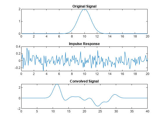
Create a signal x that has a Gaussian shape. Convolve this signal with an impulse response h that consists of random noise.

N = 200; n = 0.1*(1:N);

rng("default") x = 2exp(-0.5((n-10)).^2); h = 0.1*randn(1,length(x)); y = conv(x,h);

Plot the original signal, the impulse response, and the convolved signal.

figure tiledlayout(3,1) nexttile plot(n,x) title("Original Signal") nexttile plot(n,h) title("Impulse Response") nexttile plot(0.1*(1:length(y)),y) title("Convolved Signal")

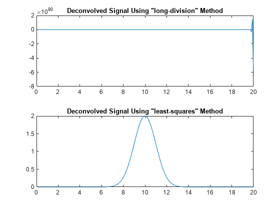
Next, find the deconvolution of signal y with respect to impulse response h using the default polynomial long-division method. Using this method, the deconvolution computation is unstable, and the result can rapidly increase.

[x1,r1] = deconv(y,h); x1(end)

Instead, find the deconvolution using the least-squares method for a numerically stable computation.

[x2,r2] = deconv(y,h,Method="least-squares");

Plot both deconvolution results. Here, the least-squares method correctly returns the original signal that has a Gaussian shape.

figure tiledlayout(2,1) nexttile plot(n,x1) title("Deconvolved Signal Using ""long-division"" Method") nexttile plot(n,x2) title("Deconvolved Signal Using ""least-squares"" Method")

Since R2023b

Create two vectors. Find the central part of the convolution of xin and h that is the same size as xin. The central part of the convolved signal y has a length of 7 instead of the full length, which is length(xin)+length(h)-1, or 10.

xin = [-1 2 3 -2 0 1 2]; h = [2 4 -1 1]; y = conv(xin,h,"same")

Find the least-squares deconvolution of signal y with respect to impulse response h. Use the "same" option to specify that the convolved signal y is only the central part, where y = conv(x,h,"same") + r. Show that deconv recovers the original signal in x within round-off error.

[x,r] = deconv(y,h,"same",Method="least-squares")

x = 1×7

-1.0000 2.0000 3.0000 -2.0000 0.0000 1.0000 2.0000

r = 1×7 10-14 ×

     0    0.0888    0.1776         0         0         0         0

Since R2023b

Create two vectors, each with two elements, and convolve them using the "valid" option. This option returns only those parts of the convolution that are computed without the zero-padded edges. In this case, the convolved signal y has only one element.

xin = [-1 2]; h = [2 5]; y = conv(xin,h,"valid")

Find the least-squares deconvolution of convolved signal y with respect to impulse response h. With the "valid" option, deconv does not always return the original signal in x, but it returns the solution of the deconvolution problem that minimizes norm(x) instead.

[x,r] = deconv(y,h,"valid",Method="least-squares")

To check the solution, you can find the full convolution of the computed signal x with h. The central part of this convolved signal is the same as the original y that defined the deconvolution problem.

yfull = 1×3

-0.3448 -1.0000 -0.3448

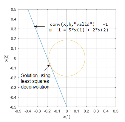
In this problem, deconv returns a different signal than the original signal because it solves for one equation with two variables, which is -1=5⋅x(1)+2⋅x(2). This system is underdetermined, meaning this system has more variables than equations. This system has infinite solutions when using the least-squares method to minimize the residual norm, or norm(y - conv(x,h,"valid")), to 0. For this reason, deconv also finds a solution that minimizes norm(x).

The following figure illustrates the situation for this underdetermined problem. The blue line represents the infinite number of solutions to the equation x(2)=-1/2-5/2⋅x(1). The orange circle represents the minimum distance from the origin to the line of solutions. The solution returned by deconv lies at the tangent point between the line and circle, indicating the solution closest to the origin.

Since R2023b

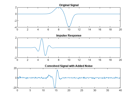
Create two signals, x and h, and convolve them. Add some random noise to the convolved signal in y.

N = 200; n = 0.1*(1:N);

rng("default") x = 2exp(-0.8(n - 8).^2) - 4exp(-2(n - 10).^2); h = 2.exp(-1(n - 5).^2).cos(4n); y = conv(x,h); y = y + max(y)0.05randn(1,length(y));

Plot the original signal, the impulse response, and the convolved signal.

figure tiledlayout(3,1) nexttile plot(n,x) title("Original Signal") nexttile plot(n,h) title("Impulse Response") nexttile plot(0.1*(1:length(y)),y) title("Convolved Signal with Added Noise")

Next, find the deconvolution of the noisy signal y with respect to the impulse response h by using the least-squares method without a regularization factor. By default, the regularization factor is 0.

[x1,r1] = deconv(y,h,Method="least-squares");

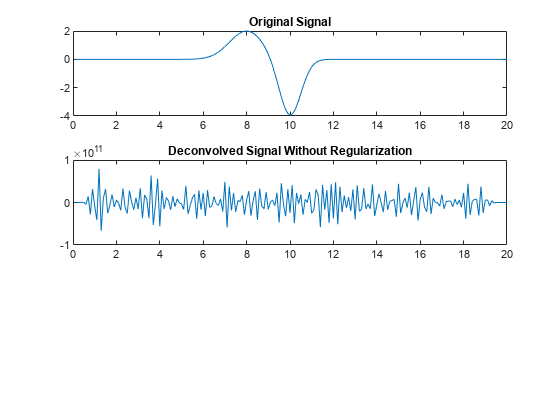
Plot the original signal and the deconvolved signal. Here, the deconv function without a regularization factor cannot recover the original signal from the noisy signal.

figure; tiledlayout(3,1); nexttile plot(n,x) title("Original Signal") nexttile plot(n,x1) title("Deconvolved Signal Without Regularization");

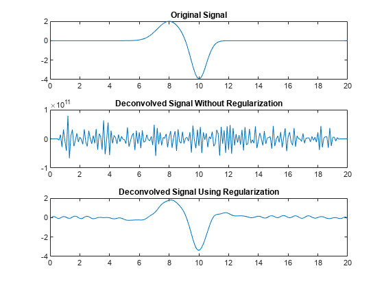
Instead, find the deconvolution of y with respect to h by using the least-squares method with a regularization factor of 1. For an ill-conditioned deconvolution problem, such as one that involves noisy signal, you can specify a regularization factor so that overfitting does not occur in the least-squares solution.

[x2,r2] = deconv(y,h,Method="least-squares",RegularizationFactor=1);

Plot this deconvolved signal. Here, the deconv function with a specified regularization factor recovers the original signal.

nexttile plot(n,x2) title("Deconvolved Signal Using Regularization")

Input Arguments

collapse all

Input signal to be deconvolved, specified as a row or column vector.

Data Types: double | single
Complex Number Support: Yes

Impulse response or filter used for deconvolution, specified as a row or column vector. y and h can have different lengths and data types.

• If one or both of y andh are of type single, then the outputs are also of type single. Otherwise, the outputs are of typedouble.
• The lengths of the inputs should satisfy length(h) <= length(y). However, if length(h) > length(y), then deconv returns the outputs as x = 0 and r = y.

Data Types: double | single
Complex Number Support: Yes

Since R2023b

Subsection of the convolved signal, specified as one of these values:

• "full" (default) — y contains the full convolution of x withh.
• "same" — y contains the central part of the convolution that is the same size asx.
• "valid" — y contains only those parts of the convolution that are computed without the zero-padded edges. Using this option,length(y) ismax(length(x)-length(h)+1,0), except whenlength(h) is zero. If length(h) = 0, then length(y) = length(x).

Name-Value Arguments

collapse all

Specify optional pairs of arguments asName1=Value1,...,NameN=ValueN, where Name is the argument name and Value is the corresponding value. Name-value arguments must appear after other arguments, but the order of the pairs does not matter.

Example: [x,r] = deconv(y,h,Method="least-squares",RegularizationFactor=1e-3)

Since R2023b

Deconvolution method, specified as one of these values:

• "long-division" — Deconvolution by polynomial long division (default).
• "least-squares" — Deconvolution by least squares, where the deconvolved signalx is computed to minimize the norm of the residual signal (or remainder) r. That is, x is the solution that minimizesnorm(y - conv(x,h)).

Since R2023b

Tikhonov regularization factor for least-squares deconvolution, specified as a real number. When using the least-squares deconvolution method, specifying the regularization factor as alpha returns a vector x that minimizes norm(r)^2 + norm(alpha*x)^2. For ill-conditioned problems, specifying the regularization factor gives preference to solutionsx with smaller norms.

If you use the default long-division deconvolution method, thenRegularizationFactor must be0.

Data Types: double | single

Output Arguments

collapse all

Deconvolved signal or quotient from division, returned as a row or column vector such that y = conv(x,h) + r.

Data Types: double | single

Residual signal or remainder from division, returned as a row or column vector such that y = conv(x,h) + r.

Data Types: double | single

References

[1] Nagy, James G. “Fast Inverse QR Factorization for Toeplitz Matrices.” SIAM Journal on Scientific Computing 14, no. 5 (September 1993): 1174–93. https://doi.org/10.1137/0914070.

Extended Capabilities

expand all

Usage notes and limitations:

• For input arguments y and h:
  • You must specify the input vector as a fixed-size or variable-length vector at code generation time. Either the first or the second dimension of the vector can be variable size. All other dimensions must have a fixed size of 1.

The deconv function supports GPU array input with these usage notes and limitations:

• Specifying impulse response or filter h as a sparsegpuArray is not supported.
• The "least-squares" deconvolution method is not supported.

For more information, see Run MATLAB Functions on a GPU (Parallel Computing Toolbox).

Version History

Introduced before R2006a

expand all

You can now perform least-squares deconvolution by specifying theMethod name-value argument as"least-squares". You can also specify different convolved subsections and the Tikhonov regularization factor with least-squares deconvolution.

In previous releases, deconv can perform deconvolution using only a polynomial long-division method. The new arguments allow you to perform least-squares deconvolution (Method="least-squares"), which returns more stable solutions compared to the default long-division deconvolution (Method="long-division").

When you use the least-squares method to deconvolve a signal y with respect to an impulse response h, deconv returns the signal x that minimizes the norm of the residual signal (or remainder) r = y - conv(x,h). That is,x is the solution that minimizes norm(r). You can also specify the Tikhonov regularization factor alpha to return a solution x that minimizes norm(r)^2 + norm(alpha*x)^2 for ill-conditioned problems.