fftshift - Shift zero-frequency component to center of spectrum - MATLAB (original) (raw)

Shift zero-frequency component to center of spectrum

Syntax

Description

Y = fftshift([X](#bviss0f-1-X)) rearranges a Fourier transform X by shifting the zero-frequency component to the center of the array.

• If X is a vector, then fftshift swaps the left and right halves of X.
• If X is a matrix, then fftshift swaps the first quadrant of X with the third, and the second quadrant with the fourth.
• If X is a multidimensional array, then fftshift swaps half-spaces of X along each dimension.

example

Y = fftshift([X](#bviss0f-1-X),[dim](#bviss0f-1-dim)) operates along the dimension dim of X. For example, if X is a matrix whose rows represent multiple 1-D transforms, then fftshift(X,2) swaps the halves of each row of X.

example

Examples

collapse all

Shift Vector Elements

Swap the left and right halves of a row vector. If a vector has an odd number of elements, then the middle element is considered part of the left half of the vector.

Xeven = [1 2 3 4 5 6]; fftshift(Xeven)

Xodd = [1 2 3 4 5 6 7]; fftshift(Xodd)

Shift 1-D Signal

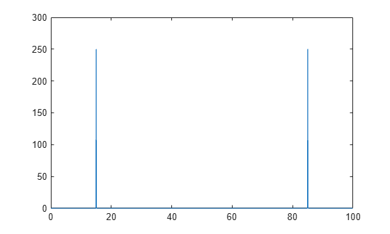
When analyzing the frequency components of signals, it can be helpful to shift the zero-frequency components to the center.

Create a signal S, compute its Fourier transform, and plot the power.

fs = 100; % sampling frequency t = 0:(1/fs):(10-1/fs); % time vector S = cos(2pi15t); n = length(S); X = fft(S); f = (0:n-1)(fs/n); %frequency range power = abs(X).^2/n; %power plot(f,power)

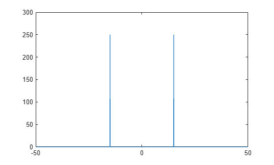
Shift the zero-frequency components and plot the zero-centered power.

Y = fftshift(X); fshift = (-n/2:n/2-1)*(fs/n); % zero-centered frequency range powershift = abs(Y).^2/n; % zero-centered power plot(fshift,powershift)

Shift Signals in Matrix

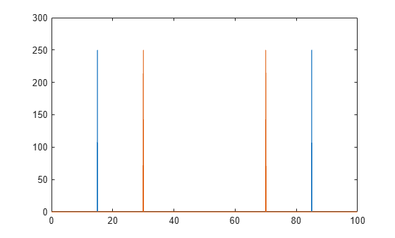
You can process multiple 1-D signals by representing them as rows in a matrix. Then use the dimension argument to compute the Fourier transform and shift the zero-frequency components for each row.

Create a matrix A whose rows represent two 1-D signals, and compute the Fourier transform of each signal. Plot the power for each signal.

fs = 100; % sampling frequency t = 0:(1/fs):(10-1/fs); % time vector S1 = cos(2pi15t); S2 = cos(2pi30t); n = length(S1); A = [S1; S2]; X = fft(A,[],2); f = (0:n-1)*(fs/n); % frequency range power = abs(X).^2/n; % power plot(f,power(1,:),f,power(2,:))

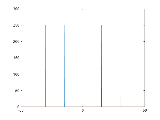
Shift the zero-frequency components, and plot the zero-centered power of each signal.

Y = fftshift(X,2); fshift = (-n/2:n/2-1)*(fs/n); % zero-centered frequency range powershift = abs(Y).^2/n; % zero-centered power plot(fshift,powershift(1,:),fshift,powershift(2,:))

Input Arguments

collapse all

X — Input array

vector | matrix | multidimensional array

Input array, specified as a vector, a matrix, or a multidimensional array.

Data Types: double | single | int8 | int16 | int32 | int64 | uint8 | uint16 | uint32 | uint64 | logical
Complex Number Support: Yes

dim — Dimension to operate along

positive integer scalar

Dimension to operate along, specified as a positive integer scalar. If no value is specified, then fftshift swaps along all dimensions.

• Consider an input matrix Xc. The operation fftshift(Xc,1) swaps halves of each column of Xc.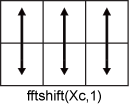
  
• Consider a matrix Xr. The operation fftshift(Xr,2) swaps halves of each row of Xr.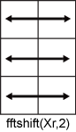
  

Data Types: double | single | int8 | int16 | int32 | int64 | uint8 | uint16 | uint32 | uint64 | logical

Extended Capabilities

C/C++ Code Generation

Generate C and C++ code using MATLAB® Coder™.

GPU Code Generation

Generate CUDA® code for NVIDIA® GPUs using GPU Coder™.

Thread-Based Environment

Run code in the background using MATLAB® backgroundPool or accelerate code with Parallel Computing Toolbox™ ThreadPool.

This function fully supports thread-based environments. For more information, see Run MATLAB Functions in Thread-Based Environment.

GPU Arrays

Accelerate code by running on a graphics processing unit (GPU) using Parallel Computing Toolbox™.

The fftshift function fully supports GPU arrays. To run the function on a GPU, specify the input data as a gpuArray (Parallel Computing Toolbox). For more information, see Run MATLAB Functions on a GPU (Parallel Computing Toolbox).

Distributed Arrays

Partition large arrays across the combined memory of your cluster using Parallel Computing Toolbox™.

This function fully supports distributed arrays. For more information, see Run MATLAB Functions with Distributed Arrays (Parallel Computing Toolbox).

Version History

Introduced before R2006a