GraphPlot - Graph plot for directed and undirected graphs - MATLAB (original) (raw)

• Documentation
• Examples
• Functions
• Apps
• Videos
• Answers

Main Content

Graph plot for directed and undirected graphs

Description

Graph plots are the primary way to visualize graphs and networks created using the graph and digraph functions. After you create a GraphPlot object, you can modify aspects of the plot by changing its property values. This is particularly useful for modifying the display of the graph nodes or edges.

Creation

To create a GraphPlot object, specify an output argument with theplot function. For example:

G = graph([1 1 1 1 5 5 5 5],[2 3 4 5 6 7 8 9]); h = plot(G)

Properties

Object Functions

Examples

collapse all

Adjust Properties of GraphPlot Object

Create a GraphPlot object, and then show how to adjust the properties of the object to affect the output display.

Create and plot a graph.

s = [1 1 1 1 1 1 1 9 9 9 9 9 9 9]; t = [2 3 4 5 6 7 8 2 3 4 5 6 7 8]; G = graph(s,t); h = plot(G)

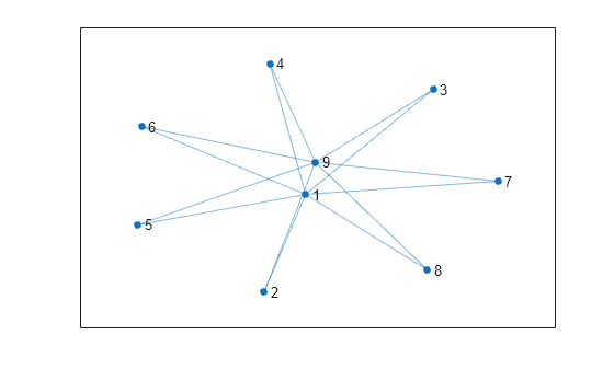
h = GraphPlot with properties:

 NodeColor: [0 0.4470 0.7410]
MarkerSize: 4
    Marker: 'o'
 EdgeColor: [0 0.4470 0.7410]
 LineWidth: 0.5000
 LineStyle: '-'
 NodeLabel: {'1'  '2'  '3'  '4'  '5'  '6'  '7'  '8'  '9'}
 EdgeLabel: {}
     XData: [-0.0552 -0.5371 1.4267 -0.4707 -2.0048 -1.9560 2.1807 1.3586 0.0577]
     YData: [-0.3011 -2.1306 1.6662 2.1447 -0.8743 0.9689 -0.0560 -1.7169 0.2991]
     ZData: [0 0 0 0 0 0 0 0 0]

Use GET to show all properties

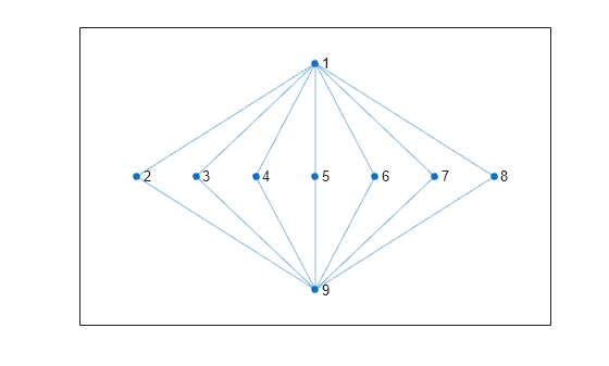
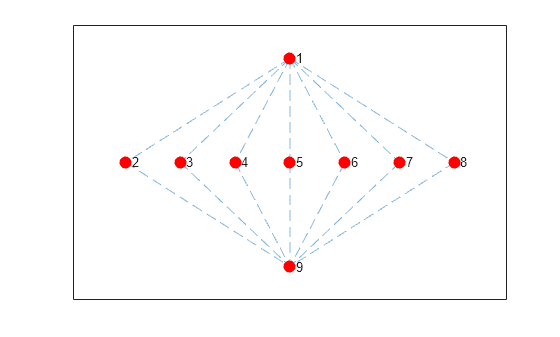
Use custom node coordinates for the graph nodes.

h.XData = [0 -3 -2 -1 0 1 2 3 0]; h.YData = [2 0 0 0 0 0 0 0 -2];

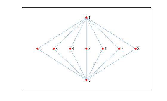
Make the graph nodes red.

Use dashed lines for the graph edges.

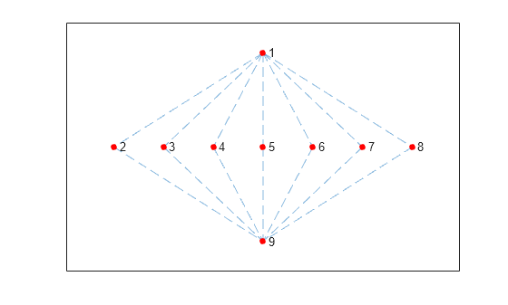
Increase the size of the nodes.

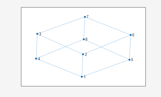
Saving and Loading GraphPlot Objects

Use the savefig function to save a graph plot figure.

s = [1 1 1 2 2 3 3 4 5 5 6 7]; t = [2 4 5 3 6 4 7 8 6 8 7 8]; G = graph(s,t); plot(G); savefig('cubegraph.fig'); clear s t G close gcf

Use openfig to load the graph plot figure back into MATLAB®. openfig also returns a handle to the figure, y.

y = openfig('cubegraph.fig');

Use the findobj function to locate the correct object handle using one of the property values. Using findobj allows you to continue manipulating the original GraphPlot object used to generate the figure.

h = findobj('Marker','o')

h = GraphPlot with properties:

 NodeColor: [0 0.4470 0.7410]
MarkerSize: 4
    Marker: 'o'
 EdgeColor: [0 0.4470 0.7410]
 LineWidth: 0.5000
 LineStyle: '-'
 NodeLabel: {'1'  '2'  '3'  '4'  '5'  '6'  '7'  '8'}
 EdgeLabel: {}
     XData: [0.3337 -1.2957 0.5299 1.9973 -0.5286 -1.9957 -0.3355 1.2947]
     YData: [0.3585 -1.2792 -2.0088 -0.5411 2.0111 0.5400 -0.3594 1.2789]
     ZData: [0 0 0 0 0 0 0 0]

Use GET to show all properties

Version History

Introduced in R2015b

expand all

R2018b: Change to default text interpreter

The new GraphPlot property Interpreter has a default value of 'tex'. In previous releases, graph node and edge labels displayed text as the literal characters instead of interpreting the text using TeX markup. If you do not want node and edge labels to use TeX markup, then set the Interpreter property to'none'.

R2018a: Self-loop display change

Self-loops in the plot of a simple graph are now shaped like a leaf or teardrop. In previous releases, self-loops were displayed as circles.