plot - Plot graph nodes and edges - MATLAB (original) (raw)
Plot graph nodes and edges
Syntax
Description
plot([G](#buofmtb-1%5Fsep%5Fshared-G)) plots the nodes and edges in graph G.
plot([G](#buofmtb-1%5Fsep%5Fshared-G),[LineSpec](#buofmtb-1-LineSpec)) sets the line style, marker symbol, and color. For example,plot(G,'-or') uses red circles for the nodes and red lines for the edges.
plot(___,[Name,Value](#namevaluepairarguments)) uses additional options specified by one or more Name-Value pair arguments using any of the input argument combinations in previous syntaxes. For example,plot(G,'Layout','circle') plots a circular ring layout of the graph, and plot(G,'XData',X,'YData',Y,'ZData',Z) specifies the(X,Y,Z) coordinates of the graph nodes.
plot([ax](#buofmtb-1-ax),___) plots into the axes specified by ax instead of into the current axes (gca). The option, ax, can precede any of the input argument combinations in previous syntaxes.
[h](#buofmtb-1-h) = plot(___) returns aGraphPlot object. Use this object to inspect and adjust the properties of the plotted graph.
Examples
Plot Graph
Create a graph using a sparse adjacency matrix, and then plot the graph.
n = 10; A = delsq(numgrid('L',n+2)); G = graph(A,'omitselfloops')
G = graph with properties:
Edges: [130x2 table]
Nodes: [75x0 table]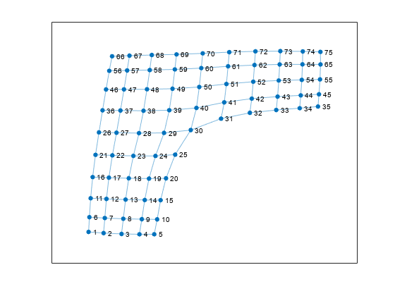
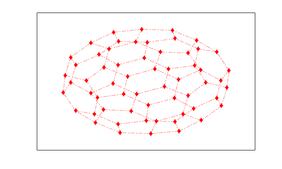
Plot Graph Using Line Specifier
Create and plot a graph. Specify the LineSpec input to change the Marker, NodeColor, and/or LineStyle of the graph plot.
G = graph(bucky); plot(G,'-.dr','NodeLabel',{})
Plot Graph with Specified Layout
Create a directed graph, and then plot the graph using the 'force' layout.
G = digraph(1,2:5); G = addedge(G,2,6:15); G = addedge(G,15,16:20)
G = digraph with properties:
Edges: [19x1 table]
Nodes: [20x0 table]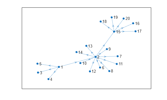
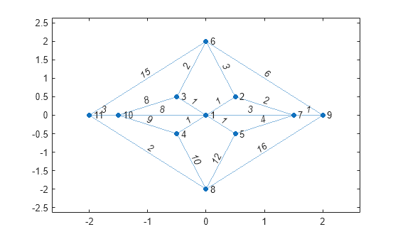
Custom Graph Node Coordinates
Create a weighted graph.
s = [1 1 1 1 1 2 2 7 7 9 3 3 1 4 10 8 4 5 6 8]; t = [2 3 4 5 7 6 7 5 9 6 6 10 10 10 11 11 8 8 11 9]; weights = [1 1 1 1 3 3 2 4 1 6 2 8 8 9 3 2 10 12 15 16]; G = graph(s,t,weights)
G = graph with properties:
Edges: [20x2 table]
Nodes: [11x0 table]
Plot the graph using custom coordinates for the nodes. The x-coordinates are specified using XData, the y-coordinates are specified using YData, and the z-coordinates are specified using ZData. Use EdgeLabel to label the edges using the edge weights.
x = [0 0.5 -0.5 -0.5 0.5 0 1.5 0 2 -1.5 -2]; y = [0 0.5 0.5 -0.5 -0.5 2 0 -2 0 0 0]; z = [5 3 3 3 3 0 1 0 0 1 0]; plot(G,'XData',x,'YData',y,'ZData',z,'EdgeLabel',G.Edges.Weight)
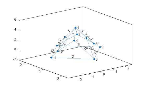
View the graph from above.
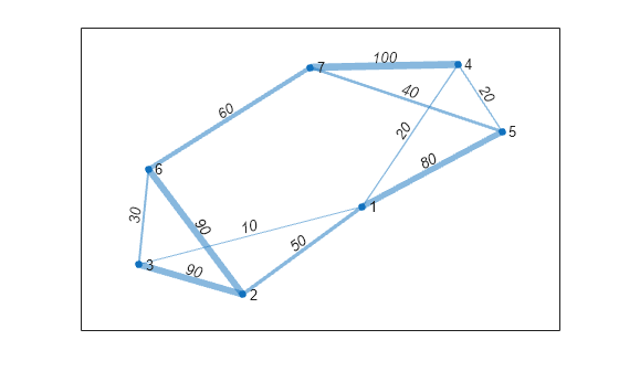
Edge Line Width Proportional to Edge Weight
Create a weighted graph.
s = [1 1 1 1 2 2 3 4 4 5 6]; t = [2 3 4 5 3 6 6 5 7 7 7]; weights = [50 10 20 80 90 90 30 20 100 40 60]; G = graph(s,t,weights)
G = graph with properties:
Edges: [11x2 table]
Nodes: [7x0 table]
Plot the graph, labeling the edges with their weights, and making the width of the edges proportional to their weights. Use a rescaled version of the edge weights to determine the width of each edge, such that the widest line has a width of 5.
LWidths = 5*G.Edges.Weight/max(G.Edges.Weight); plot(G,'EdgeLabel',G.Edges.Weight,'LineWidth',LWidths)
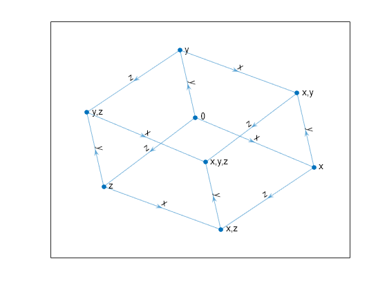
Label Graph Nodes and Edges
Create a directed graph. Plot the graph with custom labels for the nodes and edges.
s = [1 1 1 2 2 3 3 4 4 5 6 7]; t = [2 3 4 5 6 5 7 6 7 8 8 8]; G = digraph(s,t)
G = digraph with properties:
Edges: [12x1 table]
Nodes: [8x0 table]
eLabels = {'x' 'y' 'z' 'y' 'z' 'x' 'z' 'x' 'y' 'z' 'y' 'x'}; nLabels = {'{0}','{x}','{y}','{z}','{x,y}','{x,z}','{y,z}','{x,y,z}'}; plot(G,'Layout','force','EdgeLabel',eLabels,'NodeLabel',nLabels)
Adjust GraphPlot Properties
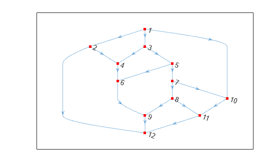
Create and plot a directed graph. Specify an output argument to plot to return a handle to the GraphPlot object.
s = [1 1 1 2 2 3 3 4 5 5 6 7 7 8 8 9 10 11]; t = [2 3 10 4 12 4 5 6 6 7 9 8 10 9 11 12 11 12]; G = digraph(s,t)
G = digraph with properties:
Edges: [18x1 table]
Nodes: [12x0 table]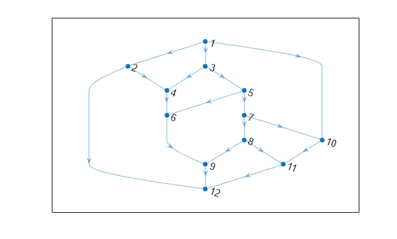
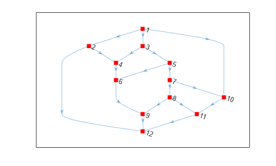
p = GraphPlot with properties:
 NodeColor: [0 0.4470 0.7410]
MarkerSize: 4
    Marker: 'o'
 EdgeColor: [0 0.4470 0.7410]
 LineWidth: 0.5000
 LineStyle: '-'
 NodeLabel: {'1'  '2'  '3'  '4'  '5'  '6'  '7'  '8'  '9'  '10'  '11'  '12'}
 EdgeLabel: {}
     XData: [2.5000 1.5000 2.5000 2 3 2 3 3 2.5000 4 3.5000 2.5000]
     YData: [7 6 6 5 5 4 4 3 2 3 2 1]
     ZData: [0 0 0 0 0 0 0 0 0 0 0 0]
Use GET to show all properties
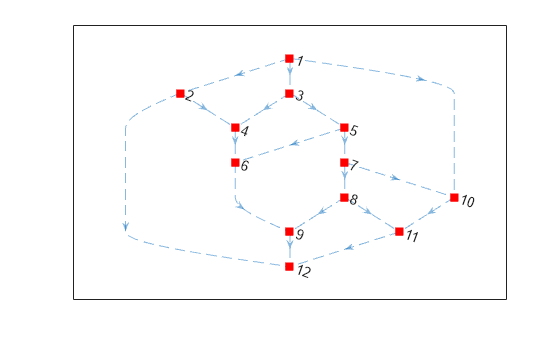
Change the color and marker of the nodes.
p.Marker = 's'; p.NodeColor = 'r';
Increase the size of the nodes.
Change the line style of the edges.
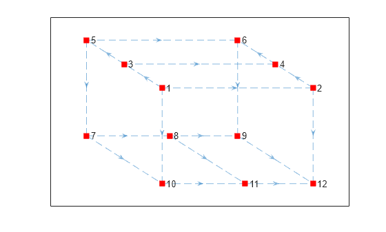
Change the x and y coordinates of the nodes.
p.XData = [2 4 1.5 3.5 1 3 1 2.1 3 2 3.1 4]; p.YData = [3 3 3.5 3.5 4 4 2 2 2 1 1 1];
Input Arguments
Input graph, specified as either a graph or digraph object. Use graph to create an undirected graph ordigraph to create a directed graph.
Example: G = graph(1,2)
Example: G = digraph([1 2],[2 3])
LineSpec — Line style, marker symbol, and color
character vector | string vector
Line style, marker symbol, and color, specified as a character vector or string vector of symbols. The symbols can appear in any order, and you can omit one or more of the characteristics. If you omit the line style, then the plot shows solid lines for the graph edges.
Example: '--or' uses red circle node markers and red dashed lines as edges.
Example: 'r*' uses red asterisk node markers and solid red lines as edges.
| Line Style | Description | Resulting Line |
|---|---|---|
| "-" | Solid line |  |
| "--" | Dashed line |  |
| ":" | Dotted line |  |
| "-." | Dash-dotted line |  |
| Marker | Description | Resulting Marker |
|---|---|---|
| "o" | Circle |  |
| "+" | Plus sign |  |
| "*" | Asterisk |  |
| "." | Point |  |
| "x" | Cross |  |
| "_" | Horizontal line |  |
| "|" | Vertical line |  |
| "square" | Square |  |
| "diamond" | Diamond |  |
| "^" | Upward-pointing triangle |  |
| "v" | Downward-pointing triangle |  |
| ">" | Right-pointing triangle |  |
| "<" | Left-pointing triangle |  |
| "pentagram" | Pentagram |  |
| "hexagram" | Hexagram |  |
| Color Name | Short Name | RGB Triplet | Appearance |
|---|---|---|---|
| "red" | "r" | [1 0 0] |  |
| "green" | "g" | [0 1 0] |  |
| "blue" | "b" | [0 0 1] |  |
| "cyan" | "c" | [0 1 1] |  |
| "magenta" | "m" | [1 0 1] |  |
| "yellow" | "y" | [1 1 0] |  |
| "black" | "k" | [0 0 0] |  |
| "white" | "w" | [1 1 1] |  |
ax — Axes object
object
Axes object. If you do not specify an axes object, thenplot uses the current axes (gca).
Name-Value Arguments
Specify optional pairs of arguments asName1=Value1,...,NameN=ValueN, where Name is the argument name and Value is the corresponding value. Name-value arguments must appear after other arguments, but the order of the pairs does not matter.
Before R2021a, use commas to separate each name and value, and enclose Name in quotes.
Example: p = plot(G,'EdgeColor','r','NodeColor','k','LineStyle','--')
The graph properties listed here are only a subset. For a complete list, seeGraphPlot Properties.
ArrowSize — Arrow size
positive value
Note
ArrowSize only affects the display of directed graphs created using digraph.
Arrow size, specified as the comma-separated pair consisting of'ArrowSize' and a positive value in point units. The default value of ArrowSize is7 for graphs with 100 or fewer nodes, and4 for graphs with more than 100 nodes.
Example: 15
EdgeCData — Color data of edge lines
vector
Color data of edge lines, specified as the comma-separated pair consisting of 'EdgeCData' and a vector with length equal to the number of edges in the graph. The values inEdgeCData map linearly to the colors in the current colormap, resulting in different colors for each edge in the plotted graph.
EdgeColor — Edge color
[0 0.4470 0.7410] (default) | RGB triplet | hexadecimal color code | color name | matrix | 'flat' | 'none'
Edge color, specified as the comma-separated pair consisting of'EdgeColor' and one of these values:
'none'— Edges are not drawn.'flat'— Color of each edge depends on the value ofEdgeCData.- matrix — Each row is an RGB triplet representing the color of one edge. The size of the matrix is
numedges(G)-by-3. - RGB triplet, hexadecimal color code, or color name — Edges use the specified color.
RGB triplets and hexadecimal color codes are useful for specifying custom colors.- An RGB triplet is a three-element row vector whose elements specify the intensities of the red, green, and blue components of the color. The intensities must be in the range
[0,1]; for example,[0.4 0.6 0.7]. - A hexadecimal color code is a character vector or a string scalar that starts with a hash symbol (
#) followed by three or six hexadecimal digits, which can range from0toF. The values are not case sensitive. Thus, the color codes"#FF8800","#ff8800","#F80", and"#f80"are equivalent.
Alternatively, you can specify some common colors by name. This table lists the named color options, the equivalent RGB triplets, and hexadecimal color codes.Color Name Short Name RGB Triplet Hexadecimal Color Code Appearance "red" "r" [1 0 0] "#FF0000" "green" "g" [0 1 0] "#00FF00" "blue" "b" [0 0 1] "#0000FF" "cyan" "c" [0 1 1] "#00FFFF" "magenta" "m" [1 0 1] "#FF00FF" "yellow" "y" [1 1 0] "#FFFF00" "black" "k" [0 0 0] "#000000" "white" "w" [1 1 1] "#FFFFFF" Here are the RGB triplets and hexadecimal color codes for the default colors MATLAB® uses in many types of plots. RGB Triplet Hexadecimal Color Code Appearance ------------------------ ---------------------- ----------------------------------------------------------------------------------------------------------------------------------------- [0 0.4470 0.7410] "#0072BD" ![Sample of RGB triplet [0 0.4470 0.7410], which appears as dark blue](https://www.mathworks.com/help/matlab/ref/colororder1.png)
[0.8500 0.3250 0.0980] "#D95319" ![Sample of RGB triplet [0.8500 0.3250 0.0980], which appears as dark orange](https://www.mathworks.com/help/matlab/ref/colororder2.png)
[0.9290 0.6940 0.1250] "#EDB120" ![Sample of RGB triplet [0.9290 0.6940 0.1250], which appears as dark yellow](https://www.mathworks.com/help/matlab/ref/colororder3.png)
[0.4940 0.1840 0.5560] "#7E2F8E" ![Sample of RGB triplet [0.4940 0.1840 0.5560], which appears as dark purple](https://www.mathworks.com/help/matlab/ref/colororder4.png)
[0.4660 0.6740 0.1880] "#77AC30" ![Sample of RGB triplet [0.4660 0.6740 0.1880], which appears as medium green](https://www.mathworks.com/help/matlab/ref/colororder5.png)
[0.3010 0.7450 0.9330] "#4DBEEE" ![Sample of RGB triplet [0.3010 0.7450 0.9330], which appears as light blue](https://www.mathworks.com/help/matlab/ref/colororder6.png)
[0.6350 0.0780 0.1840] "#A2142F" ![Sample of RGB triplet [0.6350 0.0780 0.1840], which appears as dark red](https://www.mathworks.com/help/matlab/ref/colororder7.png)
- An RGB triplet is a three-element row vector whose elements specify the intensities of the red, green, and blue components of the color. The intensities must be in the range
Example: plot(G,'EdgeColor','r') creates a graph plot with red edges.
EdgeLabel — Edge labels
{} (default) | vector | cell array of character vectors | string array
Edge labels, specified as the comma-separated pair consisting of'EdgeLabel' and a numeric vector, cell array of character vectors, or string array. The length ofEdgeLabel must be equal to the number of edges in the graph. By default EdgeLabel is an empty cell array (no edge labels are displayed).
Example: {'A', 'B', 'C'}
Example: [1 2 3]
Example: plot(G,'EdgeLabel',G.Edges.Weight) labels the graph edges with their weights.
Data Types: single | double | int8 | int16 | int32 | int64 | uint8 | uint16 | uint32 | uint64 | cell | string
Layout — Graph layout method
'auto' (default) | 'circle' | 'force' | 'layered' | 'subspace' | 'force3' | 'subspace3'
Graph layout method, specified as the comma-separated pair consisting of 'Layout' and one of the options in the table. The table also lists compatible name-value pairs to further refine each layout method. See the layout reference page for more information on these layout-specific name-value pairs.
| Option | Description | Layout-Specific Name-Value Pairs |
|---|---|---|
| 'auto' (default) | Automatic choice of layout method based on the size and structure of the graph. | — |
| 'circle' | Circular layout. Places the graph nodes on a circle centered at the origin with radius 1. | 'Center' — Center node in circular layout |
| 'force' | Force-directed layout [1]. Uses attractive forces between adjacent nodes and repulsive forces between distant nodes. | 'Iterations' — Number of force-directed layout iterations'WeightEffect' — Effect of edge weights on layout'UseGravity' — Gravity toggle for layouts with multiple components'XStart' — Starting _x_-coordinates for nodes'YStart' — Starting _y_-coordinates for nodes |
| 'layered' | Layered node layout [2], [3], [4]. Places the graph nodes into a set of layers, revealing hierarchical structure. By default the layers progress downwards (the arrows of a directed acyclic graph point down). | 'Direction' — Direction of layers'Sources' — Nodes to include in the first layer'Sinks' — Nodes to include in the last layer'AssignLayers' — Layer assignment method |
| 'subspace' | Subspace embedding node layout [5]. Plots the graph nodes in a high-dimensional embedded subspace, and then projects the positions back into 2-D. By default the subspace dimension is either 100 or the total number of nodes, whichever is smaller. | 'Dimension' — Dimension of embedded subspace |
| 'force3' | 3-D force-directed layout. | 'Iterations' — Number of force-directed layout iterations'WeightEffect' — Effect of edge weights on layout'UseGravity' — Gravity toggle for layouts with multiple components'XStart' — Starting _x_-coordinates for nodes'YStart' — Starting _y_-coordinates for nodes'ZStart' — Starting _z_-coordinates for nodes |
| 'subspace3' | 3-D subspace embedding layout. | 'Dimension' — Dimension of embedded subspace |
Example: plot(G,'Layout','force3','Iterations',10)
Example: plot(G,'Layout','subspace','Dimension',50)
Example: plot(G,'Layout','layered')
LineStyle — Line style
'-' (default) | '--' | ':' | '-.' | 'none' | cell array | string vector
Line style, specified as the comma-separated pair consisting of'LineStyle' and one of the line styles listed in this table, or as a cell array or string vector of such values. Specify a cell array of character vectors or string vector to use different line styles for each edge.
| Character(s) | Line Style | Resulting Line |
|---|---|---|
| '-' | Solid line | |
| '--' | Dashed line | |
| ':' | Dotted line | |
| '-.' | Dash-dotted line | |
| 'none' | No line | No line |
LineWidth — Edge line width
0.5 (default) | positive value | vector
Edge line width, specified as the comma-separated pair consisting of'LineWidth' and a positive value in point units or a vector of such values. Specify a vector to use a different line width for each edge in the graph.
Example: 0.75
Marker — Node marker symbol
'o' (default) | character vector | cell array | string vector
Node marker symbol, specified as the comma-separated pair consisting of 'Marker' and one of the character vectors listed in this table, or as a cell array or string vector of such values. The default is to use circular markers for the graph nodes. Specify a cell array of character vectors or string vector to use different markers for each node.
| Marker | Description | Resulting Marker |
|---|---|---|
| "o" | Circle | |
| "+" | Plus sign | |
| "*" | Asterisk | |
| "." | Point | |
| "x" | Cross | |
| "_" | Horizontal line | |
| "|" | Vertical line | |
| "square" | Square | |
| "diamond" | Diamond | |
| "^" | Upward-pointing triangle | |
| "v" | Downward-pointing triangle | |
| ">" | Right-pointing triangle | |
| "<" | Left-pointing triangle | |
| "pentagram" | Pentagram | |
| "hexagram" | Hexagram | |
| "none" | No markers | Not applicable |
Example: '+'
Example: 'diamond'
MarkerSize — Node marker size
positive value | vector
Node marker size, specified as the comma-separated pair consisting of'MarkerSize' and a positive value in point units or as a vector of such values. Specify a vector to use different marker sizes for each node in the graph. The default value ofMarkerSize is 4 for graphs with 100 or fewer nodes, and 2 for graphs with more than 100 nodes.
Example: 10
NodeCData — Color data of node markers
vector
Color data of node markers, specified as the comma-separated pair consisting of 'NodeCData' and a vector with length equal to the number of nodes in the graph. The values inNodeCData map linearly to the colors in the current colormap, resulting in different colors for each node in the plotted graph.
NodeColor — Node color
[0 0.4470 0.7410] (default) | RGB triplet | hexadecimal color code | color name | matrix | 'flat' | 'none'
Node color, specified as the comma-separated pair consisting of'NodeColor' and one of these values:
'none'— Nodes are not drawn.'flat'— Color of each node depends on the value ofNodeCData.- matrix — Each row is an RGB triplet representing the color of one node. The size of the matrix is
numnodes(G)-by-3. - RGB triplet, hexadecimal color code, or color name — Nodes use the specified color.
RGB triplets and hexadecimal color codes are useful for specifying custom colors.- An RGB triplet is a three-element row vector whose elements specify the intensities of the red, green, and blue components of the color. The intensities must be in the range
[0,1]; for example,[0.4 0.6 0.7]. - A hexadecimal color code is a character vector or a string scalar that starts with a hash symbol (
#) followed by three or six hexadecimal digits, which can range from0toF. The values are not case sensitive. Thus, the color codes"#FF8800","#ff8800","#F80", and"#f80"are equivalent.
Alternatively, you can specify some common colors by name. This table lists the named color options, the equivalent RGB triplets, and hexadecimal color codes.Color Name Short Name RGB Triplet Hexadecimal Color Code Appearance "red" "r" [1 0 0] "#FF0000" "green" "g" [0 1 0] "#00FF00" "blue" "b" [0 0 1] "#0000FF" "cyan" "c" [0 1 1] "#00FFFF" "magenta" "m" [1 0 1] "#FF00FF" "yellow" "y" [1 1 0] "#FFFF00" "black" "k" [0 0 0] "#000000" "white" "w" [1 1 1] "#FFFFFF" Here are the RGB triplets and hexadecimal color codes for the default colors MATLAB uses in many types of plots. RGB Triplet Hexadecimal Color Code Appearance ------------------------ ---------------------- ----------------------------------------------------------------------------------------------------------------------------------------- [0 0.4470 0.7410] "#0072BD" [0.8500 0.3250 0.0980] "#D95319" [0.9290 0.6940 0.1250] "#EDB120" [0.4940 0.1840 0.5560] "#7E2F8E" [0.4660 0.6740 0.1880] "#77AC30" [0.3010 0.7450 0.9330] "#4DBEEE" [0.6350 0.0780 0.1840] "#A2142F"
- An RGB triplet is a three-element row vector whose elements specify the intensities of the red, green, and blue components of the color. The intensities must be in the range
Example: plot(G,'NodeColor','k') creates a graph plot with black nodes.
NodeLabel — Node labels
node IDs (default) | vector | cell array of character vectors | string array
Node labels, specified as the comma-separated pair consisting of'NodeLabel' and a numeric vector, cell array of character vectors, or string array. The length ofNodeLabel must be equal to the number of nodes in the graph. By default NodeLabel is a cell array containing the node IDs for the graph nodes:
- For nodes without names (that is,
G.Nodesdoes not contain aNamevariable), the node labels are the valuesunique(G.Edges.EndNodes)contained in a cell array. - For named nodes, the node labels are
G.Nodes.Name'.
Example: {'A', 'B', 'C'}
Example: [1 2 3]
Example: plot(G,'NodeLabel',G.Nodes.Name) labels the nodes with their names.
Data Types: single | double | int8 | int16 | int32 | int64 | uint8 | uint16 | uint32 | uint64 | cell | string
XData — x-coordinate of nodes
vector
Note
XData and YData must be specified together so that each node has a valid (x,y) coordinate. Optionally, you can also specify ZData for 3-D coordinates.
x-coordinate of nodes, specified as the comma-separated pair consisting of 'XData' and a vector with length equal to the number of nodes in the graph.
YData — y-coordinate of nodes
vector
Note
XData and YData must be specified together so that each node has a valid (x,y) coordinate. Optionally, you can also specify ZData for 3-D coordinates.
y-coordinate of nodes, specified as the comma-separated pair consisting of 'YData' and a vector with length equal to the number of nodes in the graph.
ZData — z-coordinate of nodes
vector
Note
XData and YData must be specified together so that each node has a valid (x,y) coordinate. Optionally, you can also specify ZData for 3-D coordinates.
z-coordinate of nodes, specified as the comma-separated pair consisting of 'ZData' and a vector with length equal to the number of nodes in the graph.
Output Arguments
h — Graph plot
GraphPlot object
Graph plot, returned as an object. For more information, see GraphPlot.
References
[1] Fruchterman, T., and E. Reingold. “Graph Drawing by Force-directed Placement.” Software — Practice & Experience. Vol. 21 (11), 1991, pp. 1129–1164.
[2] Gansner, E., E. Koutsofios, S. North, and K.-P Vo. “A Technique for Drawing Directed Graphs.” IEEE Transactions on Software Engineering. Vol.19, 1993, pp. 214–230.
[3] Barth, W., M. Juenger, and P. Mutzel. “Simple and Efficient Bilayer Cross Counting.” Journal of Graph Algorithms and Applications. Vol.8 (2), 2004, pp. 179–194.
[4] Brandes, U., and B. Koepf. “Fast and Simple Horizontal Coordinate Assignment.” LNCS. Vol. 2265, 2002, pp. 31–44.
[5] Y. Koren. “Drawing Graphs by Eigenvectors: Theory and Practice.” Computers and Mathematics with Applications. Vol. 49, 2005, pp. 1867–1888.
Version History
Introduced in R2015b
R2018a: Self-loop display change
Self-loops in the plot of a simple graph are now shaped like a leaf or teardrop. In previous releases, self-loops were displayed as circles.