Normalize Data - Center and scale data in the Live Editor - MATLAB (original) (raw)
Center and scale data in the Live Editor
Since R2021b
Description
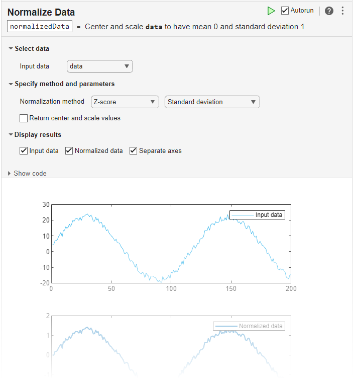
The Normalize Data task lets you interactively normalize data by choosing centering and scaling methods, such as _z_-score. The task automatically generates MATLAB® code for your live script.
Using this task, you can:
- Customize how to center and scale data in a workspace variable such as a table or timetable.
- Visualize the input data compared to the normalized data.
- Return the centering and scaling values used to compute the normalization.
More
Related Functions
Normalize Data generates code that uses the normalize function.
Open the Task
To add the Normalize Data task to a live script in the MATLAB Editor:
- On the Live Editor tab, select > .
- In a code block in the script, type a relevant keyword, such as
normalize,range, orscale. SelectNormalize Datafrom the suggested command completions. For some keywords, the task automatically updates one or more corresponding parameters.
Examples
Normalize Multiple Data Sets with Same Parameters
Interactively normalize a data set and return the computed parameter values using the Normalize Data task in the Live Editor. Then, reuse the parameters to apply the same normalization to another data set.
Create a timetable with two variables: Temperature and WindSpeed. Then create a second timetable with the same variables, but with the samples taken a year later.
Time1 = (datetime(2019,1,1):days(1):datetime(2019,1,10))'; Temperature = randi([10 40],10,1); WindSpeed = randi([0 20],10,1); T1 = timetable(Temperature,WindSpeed,RowTimes=Time1)
T1=10×2 timetable Time Temperature WindSpeed ___________ ___________ _________
01-Jan-2019        35             3
02-Jan-2019        38            20
03-Jan-2019        13            20
04-Jan-2019        38            10
05-Jan-2019        29            16
06-Jan-2019        13             2
07-Jan-2019        18             8
08-Jan-2019        26            19
09-Jan-2019        39            16
10-Jan-2019        39            20
Time2 = (datetime(2020,1,1):days(1):datetime(2020,1,10))'; Temperature = randi([10 40],10,1); WindSpeed = randi([0 20],10,1); T2 = timetable(Temperature,WindSpeed,RowTimes=Time2)
T2=10×2 timetable Time Temperature WindSpeed ___________ ___________ _________
01-Jan-2020 30 14
02-Jan-2020 11 0
03-Jan-2020 36 5
04-Jan-2020 38 0
05-Jan-2020 31 2
06-Jan-2020 33 17
07-Jan-2020 33 14
08-Jan-2020 22 6
09-Jan-2020 30 19
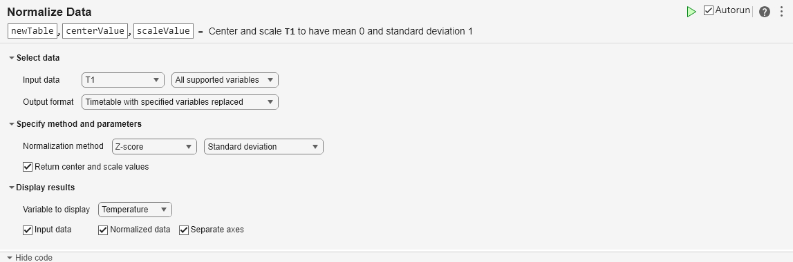
10-Jan-2020 15 0 Open the Normalize Data task in the Live Editor. To normalize the first timetable, select T1 as the input data and normalize all supported variables.
By default, the Normalize Data task returns the normalized data. In addition to the normalized data, return the centering and scaling parameter values that the task uses to perform the normalization by selecting Return center and scale values in the Specify method and parameters section of the task.
The output arguments newTable, centerValue, and scaleValue represent the normalized values, the centering values, and the scaling values, respectively.
 % Normalize Data
[newTable,centerValue,scaleValue] = normalize(T1);
% Normalize Data
[newTable,centerValue,scaleValue] = normalize(T1);
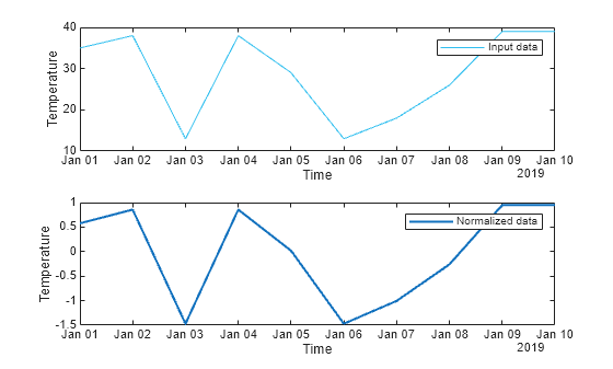
% Display results figure tiledlayout(2,1); nexttile plot(T1.Time,T1.Temperature,"SeriesIndex",6,"DisplayName","Input data") legend ylabel("Temperature") xlabel("Time")
nexttile plot(T1.Time,newTable.Temperature,"SeriesIndex",1,"LineWidth",1.5, ... "DisplayName","Normalized data") legend ylabel("Temperature") xlabel("Time")
set(gcf,"NextPlot","New")
You can use the output arguments of a Live Editor task in subsequent code. Use the normalize function to normalize the second timetable T2 using the parameter values from the first normalization. This technique ensures that the data in T2 is centered and scaled in the same way as T1.
T2_norm = normalize(T2,"center",centerValue,"scale",scaleValue)
T2_norm=10×2 timetable Time Temperature WindSpeed ___________ ___________ _________
01-Jan-2020      0.11165      0.084441
02-Jan-2020      -1.6562       -1.8858
03-Jan-2020      0.66992       -1.1822
04-Jan-2020        0.856       -1.8858
05-Jan-2020       0.2047       -1.6044
06-Jan-2020      0.39078       0.50665
07-Jan-2020      0.39078      0.084441
08-Jan-2020      -0.6327       -1.0414
09-Jan-2020      0.11165       0.78812
10-Jan-2020       -1.284       -1.8858
Related Examples
Parameters
Input data — Valid input data from workspace
vector | table | timetable
This task operates on input data contained in a vector, table, or timetable. The data can be of type single or double.
For table or timetable input data, to clean all variables with typesingle or double, select All supported variables. To choose which single ordouble variables to clean, select Specified variables.
Normalization method — Method and parameters for normalizing data
Z-score | Norm | Range | ...
Specify the method and related parameters for normalizing data as one of these options.
| Method | Method Parameters | Description |
|---|---|---|
| Z-score | Standard deviation | Center and scale to have mean 0 and standard deviation 1. |
| Median absolute deviation | Center and scale to have median 0 and median absolute deviation 1. | |
| Norm | Positive numeric scalar (default is 2) orInf for infinity norm | Scale data by _p_-norm. |
| Range | Upper and lower range limits (default is 0 for lower limit and 1 for upper limit) | Rescale range of data to an interval of the form [a, b], where a < b. |
| Median IQR | Not applicable | Center and scale data to have median 0 and interquartile range 1. |
| Center | Mean (default) | Center to have mean 0. |
| Median | Center to have median 0. | |
| Numeric scalar | Shift center by a specified numeric value. | |
| From workspace | Shift center using values in a numeric array or in a table whose variable names match the specified table variables from the input data. | |
| Scale | Standard deviation (default) | Scale data by standard deviation. |
| Median absolute deviation | Scale data by median absolute deviation. | |
| First element | Scale data by first element of data. | |
| Interquartile range | Scale data by interquartile range. | |
| Numeric scalar (default is 1) | Scale data by dividing by a specified numeric value. | |
| From workspace | Scale data using values in a numeric array or in a table whose variable names match the specified table variables from the input data. | |
| Center and scale | See the Center and Scale method parameters | Both center and scale data using the specified parameters. |
More About
_Z_-Score
For a random variable X with mean μ and standard deviation σ, the _z_-score of a value x is z=(x−μ)σ. For sample data with mean X¯ and standard deviation S, the_z_-score of a data point x is z=(x−X¯)S.
_z_-scores measure the distance of a data point from the mean in terms of the standard deviation. The standardized data set has mean 0 and standard deviation 1, and it retains the shape properties of the original data set (same skewness and kurtosis).
Median Absolute Deviation
The median absolute deviation (MAD) of a data set is the median value of the absolute deviations from the median X˜ of the data: MAD=median(|x−X˜|). Therefore, the MAD describes the variability of the data in relation to the median.
The MAD is generally preferred over using the standard deviation of the data when the data contains outliers. The standard deviation squares deviations from the mean, giving outliers an unduly large impact. Conversely, the deviations of a small number of outliers do not affect the MAD.
_P_-Norm
The general definition for the p_-norm of a vector_v that has N elements is
where p is any positive real value orInf. For common values of p:
- If p is 1, then the resulting 1-norm is the sum of the absolute values of the vector elements.
- If p is 2, then the resulting 2-norm is the vector magnitude or Euclidean length of the vector.
- If p is
Inf, then ‖v‖∞=maxi(|v(i)|).
Rescaling
Rescaling changes the distance between the minimum and maximum values in a data set by stretching or squeezing the points along the number line. The_z_-scores of the data are preserved, so the shape of the distribution remains the same.
The equation for rescaling data X to an arbitrary interval [a, b] is
Interquartile Range
The interquartile range (IQR) of a data set describes the range of the middle 50% of values when the values are sorted. If the median of the data is_Q2_, the median of the lower half of the data is Q1, and the median of the upper half of the data is Q3, then IQR = Q3 - Q1.
The IQR is generally preferred over looking at the full range of the data when the data contains outliers because the IQR excludes the largest 25% and smallest 25% of values in the data.
Version History
Introduced in R2021b
R2022b: Plot multiple table variables
Simultaneously plot multiple table variables in the display of this Live Editor task. For table or timetable data, to visualize all selected table variables at once in a tiled chart layout, set the field.
R2022b: Append normalized variables
Append input table variables with table variables containing normalized data. For table or timetable input data, to append the normalized data, set the field.
R2022a: Live Editor task does not run automatically if inputs have more than 1 million elements
This Live Editor task does not run automatically if the inputs have more than 1 million elements. In previous releases, the task always ran automatically for inputs of any size. If the inputs have a large number of elements, then the code generated by this task can take a noticeable amount of time to run (more than a few seconds).
When a task does not run automatically, the Autorun indicator is disabled. You can either run the task manually when needed or choose to enable the task to run automatically.