xspectrogram - Cross-spectrogram using short-time Fourier transforms - MATLAB (original) (raw)

Cross-spectrogram using short-time Fourier transforms

Syntax

Description

[s](#bvhos3f-s) = xspectrogram([x](#bvhos3f-x),[y](#bvhos3f-x)) returns the cross-spectrogram of the signals specified by x and y. The input signals must be vectors with the same number of elements. Each column of s contains an estimate of the short-term, time localized frequency content common tox and y.

[s](#bvhos3f-s) = xspectrogram([x](#bvhos3f-x),[y](#bvhos3f-x),[window](#bvhos3f-window)) uses window to divide x andy into segments and perform windowing.

[s](#bvhos3f-s) = xspectrogram([x](#bvhos3f-x),[y](#bvhos3f-x),[window](#bvhos3f-window),[noverlap](#bvhos3f-noverlap)) uses noverlap samples of overlap between adjoining segments.

[s](#bvhos3f-s) = xspectrogram([x](#bvhos3f-x),[y](#bvhos3f-x),[window](#bvhos3f-window),[noverlap](#bvhos3f-noverlap),[nfft](#bvhos3f-nfft)) uses nfft sampling points to calculate the discrete Fourier transform.

example

[[s](#bvhos3f-s),[w](xspectrogram.html#bvhos3f-w),[t](xspectrogram.html#bvhos3f-t)] = xspectrogram(___) returns a vector of normalized frequencies, w, and a vector of time instants, t, at which the cross-spectrogram is computed. This syntax can include any combination of input arguments from previous syntaxes.

[[s](#bvhos3f-s),[f](xspectrogram.html#bvhos3f-f),[t](xspectrogram.html#bvhos3f-t)] = xspectrogram(___,[fs](#bvhos3f-fs)) returns a vector of frequencies, f, expressed in terms offs, the sample rate. fs must be the sixth input to xspectrogram. To input a sample rate and still use the default values of the preceding optional arguments, specify these arguments as empty, [].

[[s](#bvhos3f-s),[w](xspectrogram.html#bvhos3f-w),[t](#bvhos3f-t)] = xspectrogram([x](#bvhos3f-x),[y](#bvhos3f-x),[window](#bvhos3f-window),[noverlap](#bvhos3f-noverlap),[w](xspectrogram.html#bvhos3f-w)) returns the cross-spectrogram at the normalized frequencies specified inw.

[[s](#bvhos3f-s),[f](xspectrogram.html#bvhos3f-f),[t](#bvhos3f-t)] = xspectrogram([x](#bvhos3f-x),[y](#bvhos3f-x),[window](#bvhos3f-window),[noverlap](#bvhos3f-noverlap),[f](xspectrogram.html#bvhos3f-f),[fs](#bvhos3f-fs)) returns the cross-spectrogram at the frequencies specified in f.

example

[___,[c](#bvhos3f-c)] = xspectrogram(___) also returns a matrix, c, containing an estimate of the time-varying complex cross-spectrum of the input signals. The cross-spectrogram,s, is the magnitude of c.

example

[___] = xspectrogram(___,[freqrange](#bvhos3f-freqrange)) returns the cross-spectrogram over the frequency range specified byfreqrange. Valid options forfreqrange are "onesided","twosided", and "centered".

example

[___] = xspectrogram(___,[Name,Value](#namevaluepairarguments)) specifies additional options using name-value arguments. Options include the minimum threshold and output time dimension.

example

[___] = xspectrogram(___,[spectrumtype](#bvhos3f-spectrumtype)) returns short-term cross power spectral density estimates ifspectrumtype is specified as "psd" and returns short-term cross power spectrum estimates ifspectrumtype is specified as"power".

xspectrogram(___) with no output arguments plots the cross-spectrogram in the current figure window.

xspectrogram(___,[freqloc](#bvhos3f-freqloc)) specifies the axis on which to plot the frequency. Specifyfreqloc as either "xaxis" or"yaxis".

Examples

collapse all

Generate two linear chirps sampled at 1 MHz for 10 milliseconds.

• The first chirp has an initial frequency of 150 kHz that increases to 350 kHz by the end of the measurement.
• The second chirp has an initial frequency of 200 kHz that increases to 300 kHz by the end of the measurement.

Add white Gaussian noise such that the signal-to-noise ratio is 40 dB.

nSamp = 10000; Fs = 1000e3; SNR = 40; t = (0:nSamp-1)'/Fs;

x1 = chirp(t,150e3,t(end),350e3); x1 = x1+randn(size(x1))*std(x1)/db2mag(SNR);

x2 = chirp(t,200e3,t(end),300e3); x2 = x2+randn(size(x2))*std(x2)/db2mag(SNR);

Compute and plot the cross-spectrogram of the two chirps. Divide the signals into 200-sample segments and window each segment with a Hamming window. Specify 80 samples of overlap between adjoining segments and a DFT length of 1024 samples.

xspectrogram(x1,x2,hamming(200),80,1024,Fs,'yaxis')

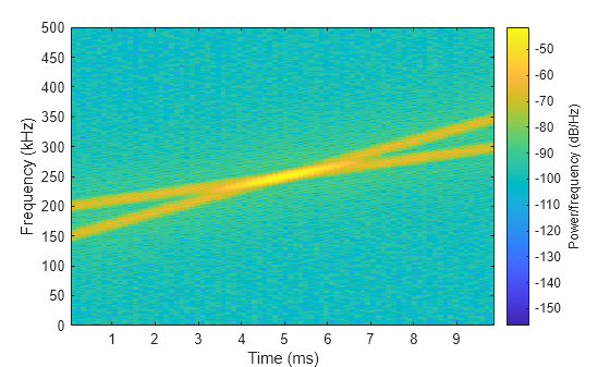
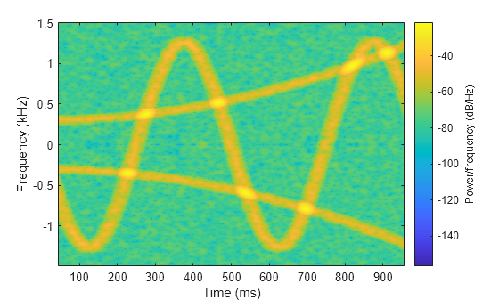
Modify the second chirp so that the frequency rises from 50 kHz to 350 kHz during the measurement. Use a 500-sample Kaiser window with shape factor β=5 to window the segments. Specify 450 samples of overlap and a DFT length of 256. Compute and plot the cross-spectrogram.

x2 = chirp(t,50e3,t(end),350e3); x2 = x2+randn(size(x2))*std(x2)/db2mag(SNR);

xspectrogram(x1,x2,kaiser(500,5),450,256,Fs,'yaxis')

In both cases, the function highlights the frequency content that the two signals have in common.

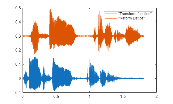
Load a file containing two speech signals sampled at 44,100 Hz.

• The first signal is a recording of a female voice saying "transform function."
• The second signal is a recording of the same female voice saying "reform justice."

Plot the two signals. Offset the second signal vertically so both are visible.

load('voice.mat')

% To hear, type soundsc(transform,fs),pause(2),soundsc(reform,fs)

t = (0:length(reform)-1)/fs;

plot(t,transform,t,reform+0.3) legend('"Transform function"','"Reform justice"')

Compute the cross-spectrogram of the two signals. Divide the signals into 1000-sample segments and window them with a Hamming window. Specify 800 samples of overlap between adjoining segments. Include only frequencies up to 4 kHz.

nwin = 1000; nvlp = 800; fint = 0:4000;

[s,f,t] = xspectrogram(transform,reform,hamming(nwin),nvlp,fint,fs);

mesh(t,f,20*log10(s)) view(2) axis tight

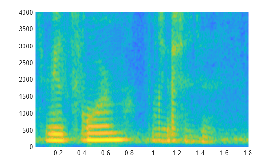
The cross-spectrogram highlights the time intervals where the signals have more frequency content in common. The syllable "form" is particularly noticeable.

Generate two quadratic chirps, each sampled at 1 kHz for 2 seconds. Both chirps have an initial frequency of 100 Hz that increases to 200 Hz midway through the measurement. The second chirp has a phase difference of 23° compared to the first.

fs = 1e3; t = 0:1/fs:2;

y1 = chirp(t,100,1,200,'quadratic',0); y2 = chirp(t,100,1,200,'quadratic',23);

Compute the complex cross-spectrogram of the chirps to extract the phase shift between them. Divide the signals into 128-sample segments. Specify 120 samples of overlap between adjoining segments. Window each segment using a Kaiser window with shape factor β = 18 and specify a DFT length of 128 samples. Use the plotting functionality of xspectrogram to display the cross-spectrogram.

[~,f,xt,c] = xspectrogram(y1,y2,kaiser(128,18),120,128,fs);

xspectrogram(y1,y2,kaiser(128,18),120,128,fs,'yaxis')

Extract and display the maximum-energy time-frequency ridge of the cross-spectrogram.

[tfr,~,lridge] = tfridge(c,f);

hold on plot(xt,tfr,'k','linewidth',2) hold off

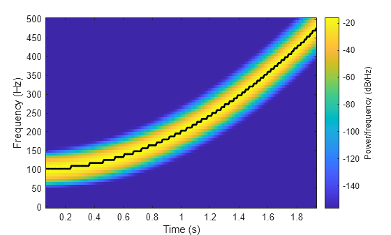
The phase shift is the ratio of imaginary part to real part of the time-varying cross-spectrum along the ridge. Compute the phase shift and express it in degrees. Display its mean value.

pshft = angle(c(lridge))*180/pi;

mean(pshft)

Generate two signals, each sampled at 3 kHz for 1 second. The first signal is a quadratic chirp whose frequency increases from 300 Hz to 1300 Hz during the measurement. The chirp is embedded in white Gaussian noise. The second signal, also embedded in white noise, is a chirp with sinusoidally varying frequency content.

fs = 3000; t = 0:1/fs:1-1/fs;

x1 = chirp(t,300,t(end),1300,'quadratic')+randn(size(t))/100;

x2 = exp(2jpi100cos(2pi2t))+randn(size(t))/100;

Compute and plot the cross-spectrogram of the two signals. Divide the signals into 256-sample segments with 255 samples of overlap between adjoining segments. Use a Kaiser window with shape factor β = 30 to window the segments. Use the default number of DFT points. Center the cross-spectrogram at zero frequency.

nwin = 256;

xspectrogram(x1,x2,kaiser(nwin,30),nwin-1,[],fs,'centered','yaxis')

Compute the power spectrum instead of the power spectral density. Set to zero the values smaller than –40 dB. Center the plot at the Nyquist frequency.

xspectrogram(x1,x2,kaiser(nwin,30),nwin-1,[],fs, ... 'power','MinThreshold',-40,'yaxis') title('Cross-Spectrogram of Quadratic Chirp and Complex Chirp')

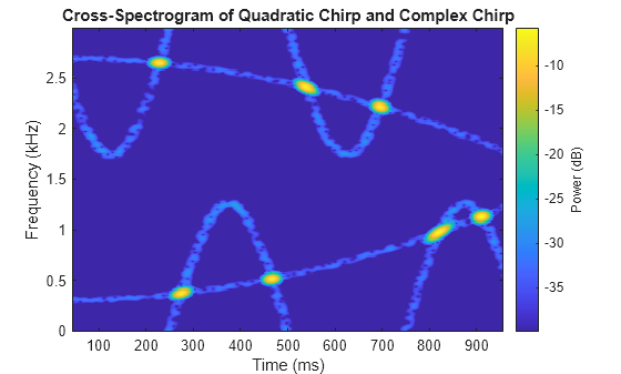
The thresholding further highlights the regions of common frequency.

Compute and plot the cross-spectrogram of two sequences.

Specify each sequence to be 4096 samples long.

To create the first sequence, generate a convex quadratic chirp embedded in white Gaussian noise and bandpass filter it.

• The chirp has an initial normalized frequency of 0.1π that increases to 0.8π by the end of the measurement.
• The 16th-order filter passes normalized frequencies between 0.2π and 0.4π rad/sample and has a stopband attenuation of 60 dB.

rx = chirp(0:N-1,0.1/2,N,0.8/2,'quadratic',[],'convex')'+randn(N,1)/100; dx = designfilt('bandpassiir','FilterOrder',16, ... 'StopbandFrequency1',0.2,'StopbandFrequency2',0.4, ... 'StopbandAttenuation',60); x = filter(dx,rx);

To create the second sequence, generate a linear chirp embedded in white Gaussian noise and bandstop filter it.

• The chirp has an initial normalized frequency of 0.9π that decreases to 0.1π by the end of the measurement.
• The 16th-order filter stops normalized frequencies between 0.6π and 0.8π rad/sample and has a passband ripple of 1 dB.

ry = chirp(0:N-1,0.9/2,N,0.1/2)'+randn(N,1)/100; dy = designfilt('bandstopiir','FilterOrder',16, ... 'PassbandFrequency1',0.6,'PassbandFrequency2',0.8, ... 'PassbandRipple',1); y = filter(dy,ry);

Plot the two sequences. Offset the second sequence vertically so both are visible.

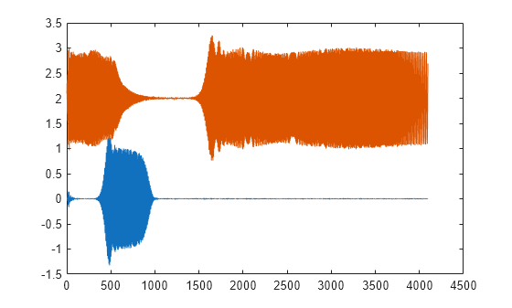
Compute and plot the cross-spectrogram of x and y. Use a 512-sample Hamming window. Specify 500 samples of overlap between adjoining segments and 2048 DFT points.

xspectrogram(x,y,hamming(512),500,2048,'yaxis')

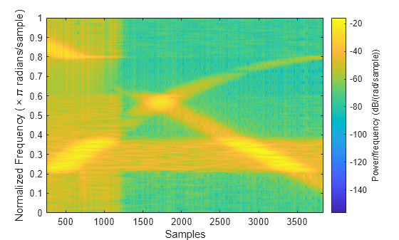
Set to zero the cross-spectrogram values smaller than –50 dB.

xspectrogram(x,y,hamming(512),500,2048,'MinThreshold',-50,'yaxis')

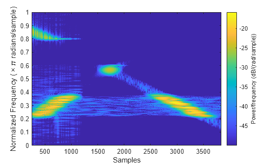
The spectrogram shows the frequency regions that are enhanced or suppressed by the filters.

Input Arguments

collapse all

Input signals, specified as vectors.

Example: cos(pi/4*(0:159))+randn(1,160) specifies a sinusoid embedded in white Gaussian noise.

Data Types: single | double
Complex Number Support: Yes

Window, specified as a positive integer or as a row or column vector. Usewindow to divide the signals into segments.

• If window is an integer, thenxspectrogram dividesx and y into segments of length window and windows each segment with a Hamming window of that length.
• If window is a vector, thenxspectrogram dividesx and y into segments of the same length as the vector and windows each segment using window.

If the input signals cannot be divided exactly into an integer number of segments with noverlap overlapping samples, then they are truncated accordingly.

If you specify window as empty, then xspectrogram uses a Hamming window such that x and y are divided into eight segments with noverlap overlapping samples.

For a list of available windows, see Windows.

Example: hann(N+1) and (1-cos(2*pi*(0:N)'/N))/2 both specify a Hann window of length N + 1.

Data Types: single | double

Number of overlapped samples, specified as a nonnegative integer.

• If window is scalar, thennoverlap must be smaller thanwindow.
• If window is a vector, thennoverlap must be smaller than the length of window.

If you specify noverlap as empty, thenxspectrogram uses a number that produces 50% overlap between segments. If the segment length is unspecified, the function sets noverlap to ⌊N/4.5⌋, where_N_ is the length of the input signals.

Data Types: double | single

Number of DFT points, specified as a positive integer. If you specifynfft as empty, thenxspectrogram sets the DFT length to max(256,2_p_), where p = ⌈log2 _Nw_⌉ and

• Nw =window if window is a scalar.
• Nw =length(`window`) if window is a vector.

Data Types: single | double

Normalized frequencies, specified as a vector. w must have at least two elements. Normalized frequencies are in rad/sample.

Example: pi./[2 4]

Data Types: double | single

Frequencies, specified as a vector. f must have at least two elements. The units of f are specified by the sample rate, fs.

Data Types: double | single

Sample rate, specified as a positive scalar. The sample rate is the number of samples per unit time. If the unit of time is seconds, then the sample rate is in Hz.

Data Types: double | single

Frequency range for the cross-spectrum estimate, specified as "onesided","twosided", or "centered". For real-valued signals, the default is "onesided". For complex-valued signals, the default is "twosided", and specifying "onesided" results in an error.

• "onesided" — Returns the one-sided cross-spectrogram of a real input signal. Ifnfft is even, then s has nfft/2 + 1 rows and is computed over the interval [0, _π_] rad/sample. If nfft is odd, then s has (nfft + 1)/2 rows and the interval is [0, _π_) rad/sample. If you specifyfs, then the intervals are respectively [0,fs/2] cycles/unit time and [0,fs/2) cycles/unit time.
• "twosided" — Returns the two-sided cross-spectrogram of a real or complex signal.s has nfft rows and is computed over the interval [0, 2_π_) rad/sample. If you specifyfs, then the interval is [0,fs) cycles/unit time.
• "centered" — Returns the centered two-sided cross-spectrogram for a real or complex signal.s has nfft rows. Ifnfft is even, then s is computed over the interval (–π,π_] rad/sample. If nfft is odd, then s is computed over (–_π,π) rad/sample. If you specifyfs, then the intervals are respectively (–fs/2, fs/2] cycles/unit time and (–fs/2,fs/2) cycles/unit time.

Data Types: char | string

Cross power spectrum scaling, specified as "psd" or"power".

• Omitting spectrumtype, or specifying"psd", returns the cross power spectral density.
• Specifying "power" scales each estimate of the cross power spectral density by the resolution bandwidth, which depends on the equivalent noise bandwidth of the window and the segment duration. The result is an estimate of the power at each frequency.

Data Types: char | string

Frequency display axis, specified as "xaxis" or "yaxis".

• "xaxis" — Displays frequency on the_x_-axis and time on the_y_-axis.
• "yaxis" — Displays frequency on the_y_-axis and time on the_x_-axis.

This argument is ignored if you callxspectrogram with output arguments.

Data Types: char | string

Name-Value Arguments

collapse all

Specify optional pairs of arguments asName1=Value1,...,NameN=ValueN, where Name is the argument name and Value is the corresponding value. Name-value arguments must appear after other arguments, but the order of the pairs does not matter.

Before R2021a, use commas to separate each name and value, and enclose Name in quotes.

Example: xspectrogram(x,100,'OutputTimeDimension',"downrows") divides x and y into segments of length 100 and windows each segment with a Hamming window of that length. The output of the spectrogram has time dimension down the rows.

Threshold, specified as a real scalar expressed in decibels.xspectrogram sets to zero those elements ofs such that 10 log10(s) ≤thresh.

Output time dimension, specified as acrosscolumns or downrows. Set this value todownrows, if you want the time dimension ofs, ps,fc, and tc down the rows and the frequency dimension along the columns. Set this value toacrosscolumns, if you want the time dimension ofs, ps,fc, and tc across the columns and frequency dimension along the rows. This input is ignored if the function is called without output arguments.

Data Types: char | string

Output Arguments

collapse all

Cross-spectrogram, returned as a matrix. Time increases across the columns of s and frequency increases down the rows, starting from zero.

• If the input signals x and y are of length N, then s has k columns, where:
  • k = ⌊(N –noverlap)/(window – noverlap)⌋ ifwindow is a scalar.
  • k = ⌊(N –noverlap)/(length(`window`) – noverlap)⌋ ifwindow is a vector.
• If the input signals are real and nfft is even, then s has (nfft/2 + 1) rows.
• If the input signals are real and nfft is odd, then s has (nfft + 1)/2 rows.
• If the input signals are complex, then s has nfft rows.

Data Types: double | single

Normalized frequencies, returned as a vector. w has a length equal to the number of rows of s.

Data Types: double | single

Time instants, returned as a vector. The time values in t correspond to the midpoint of each segment specified using window.

Data Types: double | single

Cyclical frequencies, returned as a vector. f has a length equal to the number of rows of s.

Data Types: double | single

Time-varying complex cross-spectrum, returned as a matrix. The cross-spectrogram, s, is the magnitude of c.

Data Types: double | single

References

[1] Mitra, Sanjit K.Digital Signal Processing: A Computer-Based Approach. 2nd Ed. New York: McGraw-Hill, 2001.

[2] Oppenheim, Alan V., and Ronald W. Schafer, with John R. Buck. Discrete-Time Signal Processing. 2nd Ed. Upper Saddle River, NJ: Prentice Hall, 1999.

Extended Capabilities

expand all

Usage notes and limitations:

• Arguments specified using name value pairs must be compile time constants.

Usage notes and limitations:

• Arguments specified using name-value arguments must be compile-time constants.
• Variable-size window must be double precision.

The xspectrogram function supports GPU array input with these usage notes and limitations:

• The window length must not be greater than nfft or the length of f.

For more information, see Run MATLAB Functions on a GPU (Parallel Computing Toolbox).

Version History

Introduced in R2017a

expand all

The xspectrogram function supports single-precision variable-size window inputs for code generation.

The xspectrogram function supports single-precision inputs and code generation for graphical processing units (GPUs). You must have MATLAB® Coder™ and GPU Coder™ to generate CUDA® code.