Scalable Molecular Dynamics with NAMD (original) (raw)
. Author manuscript; available in PMC: 2008 Jul 26.
Published in final edited form as: J Comput Chem. 2005 Dec;26(16):1781–1802. doi: 10.1002/jcc.20289
Abstract
NAMD is a parallel molecular dynamics code designed for high-performance simulation of large biomolecular systems. NAMD scales to hundreds of processors on high-end parallel platforms, as well as tens of processors on low-cost commodity clusters, and also runs on individual desktop and laptop computers. NAMD works with AMBER and CHARMM potential functions, parameters, and file formats. This paper, directed to novices as well as experts, first introduces concepts and methods used in the NAMD program, describing the classical molecular dynamics force field, equations of motion, and integration methods along with the efficient electrostatics evaluation algorithms employed and temperature and pressure controls used. Features for steering the simulation across barriers and for calculating both alchemical and conformational free energy differences are presented. The motivations for and a roadmap to the internal design of NAMD, implemented in C++ and based on Charm++ parallel objects, are outlined. The factors affecting the serial and parallel performance of a simulation are discussed. Next, typical NAMD use is illustrated with representative applications to a small, a medium, and a large biomolecular system, highlighting particular features of NAMD, e.g., the Tcl scripting language. Finally, the paper provides a list of the key features of NAMD and discusses the benefits of combining NAMD with the molecular graphics/sequence analysis software VMD and the grid computing/collaboratory software BioCoRE. NAMD is distributed free of charge with source code at www.ks.uiuc.edu.
Keywords: biomolecular simulation, molecular dynamics, parallel computing
1 Introduction
The life sciences enjoy today an ever-increasing wealth of information on the molecular foundation of living cells as new sequences and atomic resolution structures are deposited in databases. While originally the domain of experts, sequence data can now be mined with relative ease through advanced bioinformatics and analysis tools. Likewise, the molecular dynamics program NAMD [1], together with its sister molecular graphics program VMD [2], seeks to bring easy-to-use tools that mine structure information to all who may benefit, from the computational expert to the laboratory experimentalist.
The increase in our knowledge of structures is not as dramatic as that of sequences, yet the number of newly deposited structures reached a record 5,000 last year. For example, the structures of pharmacologically crucial membrane proteins, which were essentially unknown ten years ago, are being resolved today at a rapid pace. Structures yield static information that can be viewed with molecular graphics software such as VMD. However, structures also hold the key to dynamic information that leads to understanding function and mechanism, intellectual guideposts for basic medical research. With NAMD we want to simplify access to dynamic information extrapolated from structures and provide a molecular modeling tool that can be used productively by a wide group of biomedical researchers, including particularly experimentalists.
On a molecular scale, the fundamental processing units in the living cell are often huge in size and function in an even larger complex environment. Striking progress has been achieved in characterizing the immense machines of the cell, such as the ribosome, at the atomic level. Advances in biomedicine demand tools to model these machines in order to understand their function and their role in maintaining the health of cells. Accordingly, the purpose of NAMD is to enable high performance classical simulation of biomolecules in realistic environments of 100,000 atoms or more. The progress made in this regard is illustrated in Fig. 1. A decade ago in its first release [3, 4], NAMD permitted simulation of a protein-DNA complex encompassing 36,000 atoms [5], one of the largest simulations carried out at the time. The most recent release permitted the simulation of a protein-DNA complex of 314,000 atoms [6]. To probe the behavior of this ten-fold larger system, the simulated period actually increased hundred-fold as well.
Figure 1.
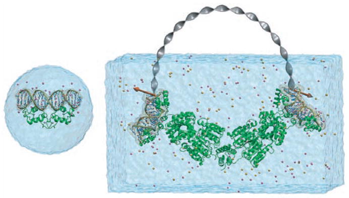
Growth in practical simulation size illustrated by comparison of estrogen receptor DNA-binding domain simulation of [5], left, 36,000 atoms simulated over 100 ps, published 1997, with multiscale LacI-DNA complex simulation of [6], right, 314,000 atoms simulated over 10 ns, published 2005 and described in Sec. 4.3.
The following article on NAMD is directed to novices and experts alike. It explains the concepts and algortithms underlying modern molecular dynamics (MD) simulations as realized in NAMD, e.g., the efficient numerical integration of the Newtonian equations of motion, the use of statistical mechanics methods for simulations that control temperature and pressure, the efficient evaluation of electrostatic forces through the particle mesh Ewald method, the use of steered and interactive MD to manipulate and probe biomolecular systems and to speed up reaction processes, and the calculation of alchemical and conformational free energy differences.
The article describes the design of NAMD and the motivation behind the design, i.e., to permit continuous software development in view of ever-changing technologies, to utilize parallel computers of any size effectively via message driven computation, to run well on platforms from laptops and desktops—where NAMD is actually used most—to parallel computers with thousands of processors. The article also demonstrates how the user can readily extend NAMD through the Tcl scripting language and elaborates on the strengths of NAMD in steered and interactive MD.
To demonstrate the broad utility of NAMD, the article introduces three typical applications as they are encountered in modern research, involving a small, an intermediate, and a large biomolecular system. We emphasize which features of NAMD were used and which were most helpful in completing the three modeling projects expeditiously. We also refer readers to tutorial material (available at http://www.ks.uiuc.edu/Training/Tutorials/) that has been proven helpful in NAMD training workshops and university courses. In fact, the first application presented below stems directly from the introductory NAMD tutorial. Other tutorials—for which a laptop provides sufficient computational power—introduce steered MD and simulations of membrane channels, as well as the use of VMD in trajectory analysis.
Finally, a conclusion section summarizes the features of NAMD that have proven to be most relevant to non-expert as well as expert users (see Table 1) and describes the great benefits that NAMD gains from its close link to the widely used molecular graphics program VMD, which permits model building as well as trajectory analysis. The integration of NAMD into the grid software BioCoRE is also mentioned.
Table 1.
Key features of NAMD.
| Ease of use: Free to download and use. Precompiled binaries provided for 12 popular platforms. Installed at major NSF supercomputer sites. Portable to virtually any platform with ethernet or MPI. C++ source code and CVS access for modification. |
|---|
| Molecule Building: Reads X-PLOR, CHARMM, AMBER, and GROMACS input files. Psfgen tool generates structure and coordinate files for CHARMM force field. Efficient conjugate gradient minimization. Fixed atoms and harmonic restraints. Thermal equilibration via periodic rescaling, reinitialization, or Langevin dynamics. |
| Basic Simulation: Constant temperature via rescaling, coupling, or Langevin dynamics. Constant pressure via Berendsen or Langevin-Hoover methods. Particle mesh Ewald full electrostatics for periodic systems. Symplectic multiple timestep integration. Rigid water molecules and bonds to hydrogen atoms. |
| Advanced Simulation: Alchemical and conformational free energy calculations. Automated pair-interaction calculations. Automated pressure profile calculations. Locally enhanced sampling via multiple images. Tcl based scripting and steering forces. Interactive visual steering interface to VMD. |
2 Molecular dynamics concepts and algorithms
In this section we outline concepts and algorithms of classical MD simulations. In these simulations the atoms of a biopolymer move according to the Newtonian equations of motion
| mαr→¨α=−∂∂r→αUtotal(r→1,r→2,…,r→N),α=1,2…N | (1) |
|---|
where mα is the mass of atom α, r⃗α is its position, and _U_total is the total potential energy that depends on all atomic positions and, thereby, couples the motion of atoms. The potential energy, represented through the MD “force field,” is the most crucial part of the simulation since it must faithfully represent the interaction between atoms yet be cast in the form of a simple mathematical function that can be calculated quickly.
Below we introduce first the functional form of the force field utilized in NAMD. We then comment on the special problem of calculating the Coulomb potential and forces efficiently. The numerical integration of (1) is then explained, followed by an outline of simulation strategies for controlling temperature and pressure. In the case of such simulations, frictional and fluctuating forces are added to (1) following the principles of non-equilibrium statistical mechanics. Finally, we describe how external, user-defined forces are added to simulations in order to manipulate and probe biomolecular systems.
2.1 Force field functions
For an all-atom MD simulation, one assumes that every atom experiences a force specified by a model force field accounting for the interaction of that atom with the rest of the system. Today, such force fields present a good compromise between accuracy and computational efficiency. NAMD employs a common potential energy function that has the following contributions:
| Utotal=Ubond+Uangle+Udihedral+UvdW+UCoulomb. | (2) |
|---|
The first three terms describe the stretching, bending, and torsional bonded interactions,
| Ubond=∑bondsikibond(ri−r0i)2; | (3) |
|---|
| Uangle=∑angleikiangle(θi−θ0i)2; | (4) |
|---|
| Udihedral=∑dihedralikidihe[1+cos(niφi−γi)] | (5) |
|---|
where bonds counts each covalent bond in the system, angles are the angles between each pair of covalent bonds sharing a single atom at the vertex, and dihedral describes atom pairs separated by exactly three covalent bonds with the central bond subject to the torsion angle φ (Fig. 2). An “improper” dihedral term governing the geometry of four planar covalently bonded atoms is also included as depicted in Fig. 2.
Figure 2.
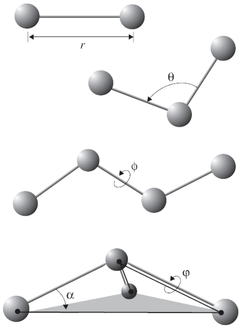
Force field bonded interactions: r governs bond stretching; θ represents the bond angle term; φ gives the dihedral angle; the out-of-plane angle α may be controlled by an “improper” dihedral ϕ.
The final two terms in 2 describe interactions between non-bonded atom pairs:
| UvdW=∑i∑j>i4εij[(σijrij)12−(σijrij)6], | (6) |
|---|
| UCoulomb=∑i∑j>iqiqj4πε0rij, | (7) |
|---|
which correspond to the van der Waal’s forces (approximated by a Lennard-Jones 6–12 potential) and electrostatic interactions, respectively.
In addition to the intrinsic potential described by the force field, NAMD also provides the user with the ability to apply external forces to the system. These forces may be used to guide the system into configurations of interest, as in steered and interactive MD (described below).
For every particle in a given context of bonds, the parameters kibond, r_0_i, etc. for the interactions given in (3–5) are laid out in force field parameter files. The determination of these parameters is a significant undertaking generally accomplished through a combination of empirical techniques and quantum mechanical calculations [7, 8, 9]; the force field is then tested for fidelity in reproducing the structural, dynamic, and thermodynamic properties of small molecules that have been well-characterized experimentally, as well as for fidelity in reproducing bulk properties. NAMD is able to use the parameterizations from both CHARMM [7] and AMBER [10] force field specifications.
In order to avoid surface effects at the boundary of the simulated system, periodic boundary conditions are often used in MD simulations; the particles are enclosed in a cell which is replicated to infinity by periodic translations. A particle which leaves the cell on one side is replaced by a copy entering the cell on the opposite side, and each particle is subject to the potential from all other particles in the system including images in the surrounding cells, thus entirely eliminating surface effects (but not finite-size effects). Because every cell is an identical copy of all the others, all the image particles move together and need only be represented once inside the molecular dynamics code.
However, because the van der Waals and electrostatic interactions (6 and 7) exist between every non-bonded pair of atoms in the system (including those in neighboring cells) computing the long-range interaction exactly is unfeasible. To perform this computation in NAMD, the van der Waals interaction is spatially truncated at a user-specified cut-off distance. For a simulation using periodic boundary conditions, the system periodicity is exploited to compute the full (non-truncated) electrostatic interaction with minimal additional cost using the particle-mesh Ewald (PME) method described in the next section.
2.2 Full electrostatic computation
Ewald summation [11] is a description of the long-range electrostatic interactions for a spatially limited system with periodic boundary conditions. The infinite sum of charge-charge interactions for a charge-neutral system is conditionally convergent, meaning that the result of the summation depends on the order it is taken. Ewald summation specifies the order as follows [12]: sum over each box first, then sum over spheres of boxes of increasingly larger radii. Ewald summation is considered more reliable than a cutoff scheme [13, 14, 15], although it is noted that the artificial periodicity can lead to bias in free energy [16, 17], and can artificially stabilize a protein which should have unfolded quickly [18].
Dropping the pre-factor 1/4_πε_, the Ewald sum involves the following terms:
| EEwald=Edir+Erec+Eself+Esurface, | (8) |
|---|
| Edir=12∑i,j=1Nqiqj∑n→r′erfc(β∣r→i−r→j+n→r∣)∣r→i−r→j+n→r∣−∑(i,j)∈Excludedqiqj∣r→i−r→j+v→ij∣, | (9) |
|---|
| Erec=12πV∑m→≠0exp(−π2∣m→∣2/β2)∣m→∣2∣∑i=1Nqiexp(2πim→⋅r→i)∣2, | (10) |
|---|
| Esurface=2π(2εs+1)V∣∑i=1Nqir→i∣2. | (12) |
|---|
Here qi and r⃗i are the charge and position of atom i, respectively, and n⃗r is the lattice vector. For an arbitrary simulation box defined by three independent base vectors _α⃗_1, _α⃗_2, _α⃗_3, one defines n⃗r = _n_1_a⃗_1 + _n_2_a⃗_2 + _n_3_a⃗_3, where _n_1, _n_2 and _n_3 are integers. Σ′ denotes a summation over n⃗r that excludes the n⃗r = 0 term in the case i = j; “Excluded” denotes the set of atom pairs whose direct electrostatic interaction should be excluded. ν⃗ij denotes the lattice vector for the (i, j) pair that minimizes |r⃗i − r⃗j + ν⃗ij|. β is a parameter adjusting the workload distribution for direct and reciprocal sums. εs is the dielectric constant of the surroundings of the simulation box, which is water for most biomolecular systems. V is the volume of the simulation box. m⃗ is the reciprocal vector defined as m⃗ = _m_1_b⃗_1 + _m_2_b⃗_2 + _m_3_b⃗_3, where _m_1, _m_2, _m_3 are integers, and the reciprocal base vectors _b⃗_1, _b⃗_2, _b⃗_3 are defined so that
| a→α.b→β=δαβ,α,β=1,2,3. | (13) |
|---|
The complementary error function erfc(x) in equation (9) is
| erfc(x)=2π∫x∞e−t2dt. | (14) |
|---|
The Ewald sum in (8) has four terms: direct sum _E_dir; reciprocal sum _E_rec; self-energy _E_self; and surface energy _E_surface. The self-energy term is a trivial constant, while the surface term is usually neglected by assuming the “tin-foil” boundary condition _ε_s = ∞, which is partly due to the dielectric constant of water (_ε_s ≈ 80) being much larger than 1. The Ewald sum has a freely chosen parameter β which can shift the computational load between the direct sum and the reciprocal sum. For a given accuracy, the computationally optimal choice of the parameter leads to a cost proportional to _N_3/2 [19] in the standard computation, where N is the number of charges in the system.
The Particle-Mesh Ewald (PME) [20] method is a fast numerical method to compute the Ewald sum. NAMD uses the smooth PME (SPME) [21] method for full electrostatic computations. The cost of PME is proportional to N log N and the time reduction is significant even for a small system of several hundred atoms. In PME, the parameter β is chosen so that the major work load is put into the reciprocal sum while the direct sum is computed by a cost proportional to N only. The reciprocal sum is then computed via fast Fourier transform (FFT) after an approximation is made to delegate the computation to a grid scheme. For this purpose, PME uses an interpolation scheme to distribute the charges, sitting anywhere in real space, to the nodes of a uniform grid as illustrated in Fig. 3. SPME uses B-spline functions as the basis functions for the interpolation. The continuity of B-spline functions and their derivatives makes the analytical expression of forces easy to obtain, and reduces the number of FFTs by half compared to the original PME method. In SPME, approximations are made to the potential only; the force is still the exact derivative of the approximated potential. The strict conservation of energy resulting from the computed force is crucial and is strongly assisted by maintaining the symplecticness of the integrator [22] as discussed further below. The PME method can be adopted to compute the electrostatic potential in real space, and has been implemented in VMD (see Fig. 4). The feature has been used recently in a ground-breaking simulation to compute trans-membrane electrostatic potentials averaged over an MD trajectory [23]. This feature makes it possible today to compute average electrostatic potentials from first principles and to replace previously used heuristic potentials like those derived from Poisson-Boltzmann theory.
Figure 3.

In PME, a charge (denoted by an empty circle with label “q”) in the figure is distributed over grid (here a mesh in two dimensions) points with weighting functions chosen according to the distance of the respective grid points to the location of the charge. Positioning all charges on a grid enables the application of the FFT method and significantly reduces the computation time. In real applications, the grid is three-dimensional.
Figure 4.
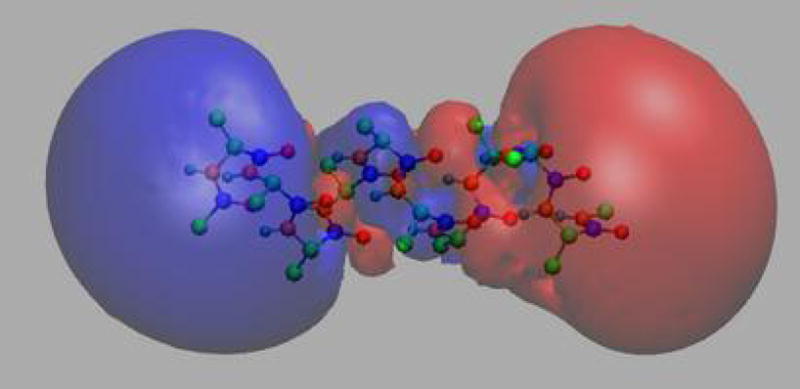
Smoothed electrostatic potential of decalanine in vacuum as calculated with the PME plugin of VMD. Atoms are colored by charge (blue is positive, red is negative). The helix dipole is clearly visible from the two potential isosurfaces +20_kBT_/e (blue, left lobe) and −20_kBT_/e (red, right lobe).
The PME method does not conserve energy and momentum simultaneously, but neither does the particle-particle-particle-mesh method [24] nor the multilevel summation method [25, 26]. Momentum conservation can be enforced by subtracting the net force from the reciprocal sum computation, albeit at the cost of a small long-time energy drift.
2.3 Numerical integration
Biomolecular simulations often require millions of timesteps. Furthermore, biological systems are chaotic; trajectories starting from slightly different initial conditions diverge exponentially fast and after a few picoseconds are completely uncorrelated. However, highly accurate trajectories are not a serious goal for biomolecular simulations; more important is a proper sampling of phase space. Therefore, for constant energy (NVE ensemble) simulations, the key features of an integrator are not only how accurate it is locally, but also how efficient it is and how well it preserves the fundamental dynamical properties, such as energy, momentum, time-reversibility, and symplecticness.
The time evolution of a strict Hamiltonian system is symplectic [22]. A consequence of this is the conservation of phase space volume along the trajectory, i.e., the enforcement of the Liouville theorem [27, page 69]. To a large extent, the trajectories computed by numerical integrators observing symplecticness represent the solution of a closely related problem that is still Hamiltonian [28]. Because of this, the errors, unavoidably generated by an integrator at each timestep, accumulate imperceptibly slowly, resulting in a very small long-time energy drift, if there is any at all [22, theorem IX.8.1]. Artificial measures to conserve energy, e.g., scaling the velocity at each timestep so that the total energy is constant, lead to biased phase space sampling of the constant energy surface [29]; in contrast, there has been no evidence that symplectic integrators have this problem.
A simple example demonstrates the merit of a symplectic integrator. For this purpose, the one-dimensional harmonic oscillator problem has been numerically integrated, the resulting trajectory being shown in Fig. 5. We note that the comparison is “unfair” to the symplectic method with respect to both accuracy (Δ_t_2 local error for the symplectic method vs. Δ_t_5 for the Runge-Kutta method, where Δ_t_ is the timestep), and computational effort (single force evaluation per timestep for the symplectic method vs. four force evaluations for the Runge-Kutta method). Nevertheless, the symplectic method shows superior long-time stability.
Figure 5.
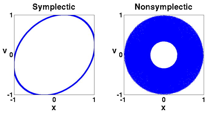
A symplectic method demonstrates superior long-time stability: the symplectic method used here is the sympletic Euler method [22, Theorem 3.3], whose local error is proportional to Δ_t_2; the non-symplectic method used is the Runge-Kutta method [30, §_8.3.3] whose local error is proportional to Δ_t_5. The system described is a one-dimension harmonic oscillator. The equation of motion is mẍ = −_mω_2_x, with m = ω = 1, and initial conditions x = 1, υ = 0. The exact trajectory is the unit circle. The chosen timestep is Δ_t_ = 0.5 and 10000 steps were integrated. The trajectory of the Runge-Kutta method collapses toward the center while the symplectic Euler method maintains a stable orbit.
NAMD uses the Verlet method [31, _§_4.2.3] for NVE ensemble simulations. The “velocity-Verlet” method obtains the position and velocity at the next timestep (rn+1, vn+1) from the current one (rn, υn), assuming the force Fn = F (rn) is already computed, in the following way:
"half−kick"vn+1/2=vn+M−1Fn⋅Δt/2,"drift"rn+1=rn+vn+1/2Δt,"computer force"Fn+1=F(rn+1),"half−kick"vn+1=vn+1/2+M−1Fn+1⋅Δt/2.
Here, M is the mass. The Verlet method is symplectic and time-reversible, conserves linear and angular momentum, and requires only one force evaluation for each timestep. For a fixed time period, the method exhibits a (global) error proportional to Δ_t_2.
More accurate (higher order) methods are desirable if they can increase the timestep per force evaluation. Higher order Runge-Kutta type methods, symplectic or not, are not suitable for biomolecular simulations since they require several force evaluations for each timestep and force evaluation is by far the most time-consuming task in molecular dynamics simulations. Gear type predictor-corrector methods [32], or linear multistep methods in general, are not symplectic [22, theorem XIV.3.1]. No symplectic method has been found as yet that is both more accurate than the Verlet method and practical for biomolecular simulations.
NAMD employs the multiple-time-stepping [33, 34, 13] method to improve integration efficiency. Because the biomolecular interactions collected in (2) generally give rise to several different timescales characteristic for biomolecular dynamics, it is natural to compute the slower-varying forces less frequently than faster-varying ones in molecular dynamics simulations. This idea is implemented in NAMD by three levels of integration loops. The inner loop uses only bonded forces to advance the system, the middle loop uses Lennard-Jones and short-range electrostatic forces, and the outer loop uses long-range electrostatic forces. It is very important that the method implemented is symplectic and time-reversible.
The longest timestep for the multiple-time-stepping method is limited by resonance [35]. When good energy conservation is needed for NVE ensemble simulations we recommend choosing 2 fs, 2 fs, and 4 fs as the inner, middle, and outer timesteps if rigid bonds to hydrogen atoms are used; or 1 fs, 1 fs, and 3 fs if bonds to hydrogen are flexible [36]. More aggressive timesteps may be used for NVT or NPT ensemble simulations, e.g., 2 fs, 2 fs, and 6 fs with rigid bonds and 1 fs, 2 fs, and 4 fs without. Using multiple-time-stepping can increase computational efficiency by a factor of 2.
2.4 NVT and NPT ensemble simulations
The fundamental requirement for an integrator is to generate the correct ensemble distribution, controlling the temperature or pressure in an appropriate way. For this purpose the Newtonian equations of motion (1) should be modified “mildly” so that the computed short-time trajectory can still be interpreted in a conventional way. In order to generate the correct ensemble distribution, the system is coupled to a reservoir, with the coupling being either deterministic or stochastic. Deterministic couplings generally have some conserved quantities (similar to total energy), the observation of which can provide some assurance about the simulation. NAMD uses a stochastic coupling approach because it is easier to implement and the friction terms tend to enhance the dynamical stability.
The (stochastic) Langevin equation [37] is used in NAMD to generate the Boltzmann distribution for canonical (NVT) ensemble simulations. The generic Langevin equation is
| Mv.=F(x)−γv−2γkBTMR(t) | (15) |
|---|
where M is the mass, υ = ẋ is the velocity, F is the force, x is the position, γ is the friction coefficient, k_B is the Boltzmann constant, T is the temperature, and R(t) is a univariate Gaussian random process. Coupling to the reservoir is modeled by adding the fluctuating (the last term) and dissipative (−_γυ term) forces to the Newtonian equations of motion (1). To integrate the Langevin equation, NAMD uses the Brünger-Brooks-Karplus (BBK) method [38], a natural extension of the Verlet method for the Langevin equation. The position recurrence relation of the BBK method is
| xn+1=xn+1−γΔt/21+γΔt/2(xn−xn−1)+11+γΔt/2Δt2[M−1F(xn)+2γkBTΔMZn] | (16) |
|---|
where Zn is a set of Gaussian random variables of zero mean and variance one. The BBK integrator requires only one random number for each degree of freedom. The steady state distribution generated by the BBK method has an error proportional to Δ_t_2 [39], although the error in the time correlation function can have an error proportional to Δ_t_ [40].
For stochastic equations of motion, position and velocity become random variables, while the time evolution of the corresponding probability distribution function is described by the Fokker-Planck equation [37, section 2.4], a deterministic partial differential equation. The stochastic equations of motion are designed so that the time-independent solution to the Fokker-Planck equation is the targeted ensemble distribution. The relationship between the Langevin equation and the associated Fokker-Planck equation has been invoked, for example, in [41]. The theory behind deterministic coupling methods is similar, with the Liouville equation playing the pivotal role [42].
For NPT ensemble simulations, one of the authors (J.P.) proposed a new set of equations of motion and implemented a numerical integrator in NAMD [43, pressure control section]. It was inspired by the Langevin-piston method [44] and Hoover’s method [45, 46, 47] for constant pressure simulations. A recent work proposed essentially the same set of equations (the “Langevin–Hoover” method given by equations (5a)–(5d) in [48]), and proved that they generate the correct ensemble distribution. The only difference between the two is the term 1 + d/Nf in equation (5b) and (5d) of [48], where d is the dimension (generally 3), and Nf is the number of degrees of freedom. The term d/Nf is small enough that NAMD simply neglects it.
2.5 Steered and interactive molecular dynamics
Biologically important events often involve transitions from one equilibrium state to another, such as the binding or dissociation of a ligand. However, processes involving the rare event of barrier crossing are difficult to reproduce on MD timescales, which today are still confined to the order of tens of nanoseconds. To address this issue, the application of external forces may be used to guide the system from one state to another, enhancing sampling along the pathway of interest. Recent applications of single-molecule experimental techniques (such as atomic force microscopy and optical tweezers) have enhanced our understanding of the mechanical properties of biopolymers. Steered molecular dynamics (SMD) is the in silico complement of such studies, in which external forces are applied to molecules in a simulation to probe their mechanical properties as well as to accelerate processes that are otherwise too slow to model. This method has been reviewed in [49, 50, 51]. With advances in available computer power, steering forces can also be applied interactively, instead of in batch-mode; we call this technique Interactive Molecular Dynamics (IMD) [52, 53]. External forces have been applied using NAMD in a variety of ways to a diverse set of systems, yielding new information about the mechanics of proteins [54], for instance in [55, 6, 56, 57, 58, 59, 60, 61, 62, 63, 64, 65, 66, 67] and other studies reviewed in [51]. We expect that most molecular dynamics simulations in the future will be of the steered type. This expectation stems from an analogy to experimental biophysics: while many experiments provide images of biological systems, more experiments investigate systems through well-designed perturbations by physical or chemical means.
SMD
Steered MD may be carried out with either a constant force applied to an atom (or set of atoms) or by attaching a harmonic (spring-like) restraint to one or more atoms in the system and then varying either the stiffness of the restraint [67] or the position of the restraint [68, 69, 70] to pull the atoms along. Other external forces or potentials can also be used, such as constant forces or torques applied to parts of the system in order to induce rotational motion of its domains. NAMD provides builtin facilities for applying a variety of external forces, including the automated application of moving constraints. In SMD, the direction of the applied force is chosen in advance, specified through a few simple lines in a NAMD configuration file. More flexible force schemes can be realized within NAMD through scripting.
As a computational technique, SMD bears similarities to the method of umbrella sampling [71, 72], which also seeks to improve the sampling of a particular degree of freedom in a biomolecular system; however, while umbrella sampling requires a series of equilibrium simulations, SMD simulations apply a constant or time-varying force which results in significant deviations from equilibrium. In consequence, the results of the SMD dynamics have to be analyzed from an explicitly nonequilibrium viewpoint [54]. SMD also permits new types of simulations which are more naturally performed and understood as out-of-equilibrium processes.
In constant force SMD, the atoms to which the force is applied are subject to a fixed, constant force in addition to the force field potential. The affected atoms are specified through a flag in the molecular coordinates (PDB) file, and the force vector is specified in the NAMD configuration. Intermediates found through constant-force SMD simulations may be modeled using the theory of mean first passage times for a barrier-crossing event [73, 74]. Typical applied forces range from tens to a thousand picoNewtons (pN) [75].
Constant velocity SMD simulates the action of a moving AFM cantilever on a protein. An atom of the protein, or the center of mass of a group of atoms, is harmonically restrained to a point in space that is then shifted in a chosen direction at a predetermined constant velocity, forcing the restrained atoms to follow (Fig. 6). By default, the SMD harmonic restraint in NAMD only applies along the direction of motion of the restraint point, such that the atoms are unrestrained along orthogonal vectors; it is possible, however, to apply additional restraints. As with constant force SMD, the affected atoms are specified through a flag in the PDB file; the force constant of the restraint and the velocity of the restraint point are specified in the NAMD configuration file. For a group of atoms harmonically restrained with a force constant k moving with velocity υ in the direction n⃗, the additional potential
Figure 6.
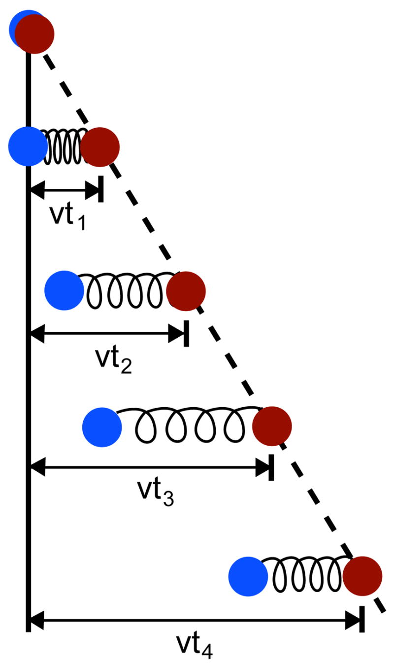
Constant velocity pulling in a one-dimensional case. The dummy atom is colored red, and the SMD atom blue. As the dummy atom moves at constant velocity, the SMD atom experiences a force that depends linearly on the distance between both atoms.
| ΔU(r→1,r→2,…,t)=12k[vt−(R→(t)−R→0)⋅n→]2 | (17) |
|---|
is applied, where R⃗(t) is the current center of mass of the SMD atoms and _R⃗_0 is their initial center of mass. n⃗ is a unit vector. In AFM experiments, the spring constants k of the cantilevers are typically of the order of 1 pN/Å, so that thermal fluctuations in the position of an attached ligand, (kBT/k)1/2, are large on the atomic scale, e.g., 6 Å. However, in SMD simulations stiffer springs (k ~70 pN/Å) are employed, leading to more detailed information about interaction energies as well as finer spatial resolution. However, due to limitations in attainable computational speeds, simulations cover time scales that are typically 105 times shorter than those of AFM experiments, necessitating high pulling velocities on the order of 1 Å/ps. As a result, a large amount of irreversible work is performed during SMD simulations, which needs to be discounted in order to obtain equilibrium information.
A proof that equilibrium properties of a system can be deduced from non-equilibrium simulations was given by Jarzynski [76, 77]. The second law of thermodynamics states that the average work 〈_W_〉 done through a non-equilibrium process that changes a parameter λ of a system from _λ_0 at time zero to λt at time t is greater than or equal to the equilibrium free energy difference between the final and initial values of λ:
where the equality holds only if the process is quasi-static. Jarzynski [76] discovered an equality that holds regardless of the speed of the process:
where β = (kBT)−1. The Jarzynski equality provides a way to extract equilibrium information, such as free energy differences, from averaging over nonequilibrium processes [76], a method that has been tested against computer simulations [77] and experiments [78].
A major difficulty that arises with the application of (19) is that the average of exponential work appearing in Jarzynski’s equality is dominated by trajectories corresponding to small work values that arise only rarely. Hence, an accurate estimate of free energy requires suitable sampling of such rare trajectories, and thus the accuracy of the method is limited by statistical error. Cumulant expansions [76, 79, 62, 41] are an effective approximation for the exponential average; since the lower-order terms of the expansion are less influenced by statistical error, the systematic error introduced by truncating the higher order terms may be considerably smaller than the statistical error which would be introduced by including them. It can be shown [41] that in the relevant regime of steering by means of stiff springs, the work on the system is Gaussian-distributed regardless of the speed of the process simulated and the cumulant expansion of Jarzynski’s equality can safely be terminated at second order [80].
Application of the Jarzynski identity (19) is comparable in efficiency to the umbrella sampling method [81]. However, the analysis involved in the SMD method is simpler than that involved in umbrella sampling in which one needs to solve coupled nonlinear equations for the weighted histogram analysis method [82, 83, 54, 31]. In addition, the application of the Jarzynski identity has the advantage of uniform sampling of a reaction coordinate. Whereas in umbrella sampling a reaction coordinate is sampled nonuniformly proportional to the Boltzmann weight, in SMD a reaction coordinate follows a guiding potential that moves with a constant velocity and, hence, is sampled almost uniformly (computing time is uniformly distributed over the given region of the reaction coordinate). This is particularly beneficial when the potential of mean force (essentially, the free energy profile along the reaction coordinate) contains narrow barrier regions as in [62]. In such cases, a successful application of umbrella sampling depends on an optimal choice of biasing potentials, whereas nonequilibrium thermodynamic integration appears to be more robust [31]. However, umbrella sampling is a general method that can be applied to a variety of reaction coordinates, including complex ones like those involved in large conformational changes in proteins [84].
NAMD also provides the facility for the user to apply other types of external forces to a system. In a technique related to SMD, torques may be applied to induce the rotation of a protein domain. As with SMD, this is implemented in NAMD through a simple specification in the configuration file and does not require additional programming on the part of the researcher. This technique has already been successfully used to study the rotation of the Fo domain of ATPase [85]. The application of more sophisticated external forces are readily implemented through the NAMD “Tcl forces” interface, which allows the user to specify position- and time-dependent forces to be computed at each time-step. This technique has recently been used to mimic the effect of membrane surface tension on a mechanosensitive channel [59] and to model the interaction of the lac repressor protein (modeled in atomic-level detail) with DNA described by an elastic rod that exerts forces on the protein [86, 6].
IMD
By using NAMD in conjunction with the molecular graphics software VMD, steering forces can be applied in an interactive manner, rather than only in batch mode [52]. For this purpose, VMD is linked to a NAMD simulation running on the same machine or a remote cluster. This arrangement permits an investigator to view a running simulation and to apply forces based on real-time information about the progress of the simulation (such as visual information or force feedback through a haptic device). The researcher is then able to explore the mechanical properties of the system in a direct, hands-on manner, using her scientific intuition to guide the simulation via a mouse or haptic device. This method has already been used in biomolecular research, for instance to study the selectivity and regulation of the membrane channel protein GlpF and the enzyme glycerol kinase [53]. Setting up an IMD simulation is a straight-forward process that can be done on any computer.
The IMD haptic interface [52] consists of three primary components: a haptic device to provide translational and orientational input as well as force feedback to the user’s hand; NAMD to calculate the effect of applied forces via molecular dynamics; and VMD to display results (Fig. 7). VMD communicates with the haptic device via a server [87] that controls the haptic environment experienced by the user, as described in [52]. The scheme of splitting the haptic, visualization, and simulation components into three communicating, asynchronous processes has been employed successfully [52, 88] and permits all three components to run at top speed, maximizing the responsiveness of the system. IMD requires efficient network communication between the visualization front-end and the MD back-end. While the network bandwidth requirements for performing IMD are quite low relative to the computational demands, latency is a major concern as it has a direct impact on the responsiveness of the system. IMD uses custom sockets code in NAMD and VMD to transfer atomic coordinates and steering forces efficiently.
Figure 7.
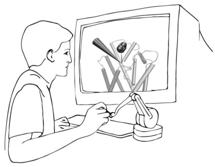
In IMD, the user applies forces to atoms in the simulation via a force-feedback haptic device.
To make molecular motion as described by MD perceptible to the IMD user through the haptic device, the quantities arising in the generic equation of motion governing the molecular response (represented below by Roman characters) and the haptic response (denoted by Greek characters),
must be related through suitable scaling factors. Molecular motion probed is typically extended over distances of x = 1 Å, molecular time scales covered are typically t = 1 ps, and external forces acting on molecular moieties should not exceed f = 1 nN in order not to overwhelm inherent molecular forces. By contrast, the haptic device is characterized by length resolution of χ = 1 cm and can generate a force of φ = 1 N or more; t = 1 ps of dynamics requires τ = 1 s or more to compute. The interface between the haptic device and NAMD thus introduces the scaling factors
| Sx=χ/x=108,St=τ/t=1012,Sf=φ/f=109, | (21) |
|---|
Multiplying the molecular equation of motion in (20) by the factor SfSx/St2 gives
| SfSxSt2md2xdt2=Sfmd2χdτ2=SfSxSt2f=SxSt2φ. | (22) |
|---|
From this we can conclude
Comparison with the haptic equation of motion in (20) suggests that the effective mass felt by the haptic device, and hence, by the user is
The molecular moieties to be moved through external forces have typical masses of (e.g., for glycerol moved through a membrane channel [53]) of m = 180 amu or m ≈ 3 × 10⁻²⁵ kg. From (21) we conclude then that the effective mass felt by the user through the haptic device is 3 kg; the user does not sense strong inertial effects and can readily manipulate the biomolecular system. IMD can also be carried out without force feedback, using a standard mouse to steer the simulated system.
To assist users of NAMD with IMD, AutoIMD [89] has been developed. AutoIMD permits the researcher to use the graphical interface provided by VMD to run an MD simulation based on a selection of atoms. The simulation can then be visualized in real-time in the VMD graphics window. Forces may be applied with either a mouse or a haptic device by the user (as described above), or statically as in traditional SMD. Rather than carrying out a simulation of the entire molecule, AutoIMD performs a rapid MD simulation by dividing the system into three parts: a “molten zone,” where the atoms are allowed to move freely; a surrounding “fixed zone,” in which the atoms are included in the simulation (and exert forces on the molten zone), but are held fixed; and an “excluded zone,” which is entirely disregarded in the AutoIMD simulation. In this way, AutoIMD may be used to inspect and perform energy minimizations on parts of the system that have been manipulated (e.g., through mutations or IMD), giving the researcher real-time feedback on the simulation.
SMD and IMD simulations differ in fundamental ways, and may be fruitfully combined. In SMD, the specification of the external forces is developed based on the researcher’s understanding of the biological and structural properties of the system. The SMD simulation is carried out with the weakest force possible to induce the necessary change in an affordable length of simulation time, and the analysis of the simulation data relates the force applied to the progress of the system along the chosen reaction path. In contrast, IMD simulations are unplanned, allowing the researcher to toy with the system, exploring the degrees of freedom. Because the simulations need to be rapid – completed in minutes rather than days or weeks – the applied forces are extremely large, and the simulations are too rough to produce data suitable for an accurate analysis of molecular properties. The techniques can be combined: in the first stage, the researcher uses IMD to generate and test hypotheses for reaction mechanisms or to accelerate substrate transport, docking, and other mechanisms that are difficult to cast into numerical descriptions; in the second stage, the researcher carries out further MD or SMD simulations using the hypothesized mechanisms or configurations from the IMD investigation.
2.6 Free energy calculations
In addition to propagating the motion of atoms in time, MD can also be used to generate an ensemble of configurations, from which thermodynamic quantities like free energy differences, Δ_F_, can be computed. In a nutshell, there are three possible routes for the calculation of Δ_F_: (i) estimate the relevant probability distribution, _ρ_[U(_r⃗_1, …, r⃗N)], from which a free energy difference may be inferred via −1/β ln _ρ_[U(r⃗_1, …, r⃗N)]/ρ_0, where ρ_0 denotes a normalization term, (ii) compute the free energy difference directly, and (iii) calculate the free energy derivative, dΔ_F (ξ)/d_ξ, over some ordering parameter, ξ, consistent with an average force [90], and integrate the latter to obtain Δ_F.
The popular umbrella sampling method [71, 72], whereby the probability to find the system along a given reaction coordinate is sought, falls evidently into the first category. One blatant shortcoming of this scheme, however, lies in the need to guess the external potential or bias that is necessary to overcome the barriers of the free energy landscape—an issue that may rapidly become intricate in the case of qualitatively new problems. In this section, we shall focus on the second and the third classes of approaches for determining free energy differences.
The first approach, available in NAMD since version 2.4, is free energy perturbation (FEP) [91], an exact method for the direct computation of relative free energies. FEP offers a convenient framework for performing “alchemical transformations”, or in silico site-directed mutagenesis of one chemical species into another.
Description of intermolecular association or intramolecular deformation in complex molecular assemblies requires an efficient computational tool, capable of rapidly providing precise free energy profiles along some ordering parameter, ξ, in particular when little is known about the underlying free energy behavior of the process. A fast and accurate scheme, pertaining to the third category of methods, is introduced in NAMD version 2.6 to determine such free energy profiles, Δ_F_ (ξ). This scheme relies upon the evaluation of the average force acting along the chosen ordering parameter, ξ, in such a way that no apparent free energy barrier impedes the progression of the system along the latter [92, 93].
The efficiency of the free energy algorithm represents only one facet of the overall performance of the free energy calculation, which, to a large extent, relies on the ability of the core MD program to supply configurations and forces in rigorous thermodynamic ensembles and in a time-bound fashion. The methodology described hereafter has been implemented in NAMD to operate synergistically with the rest of the code and at virtually no extra cost over a standard MD simulation.
Alchemical transformations
Contrary to the worthless piece of lead in the hands of the proverbial alchemist, the potential energy function of the computational chemist is sufficiently malleable to be altered seamlessly, thereby allowing the thermodynamic properties of a system to be related to those of a slightly modified one, such as a chemically modified protein or ligand, through the difference in the corresponding intermolecular potentials.
The free energy difference between a reference state, a, and a target state, b, can be expressed in terms of the ratio of their corresponding partition functions:
| ΔFa→b=−1βln∫exp[−βUb(r→1,…,r→N)]dr→1…dr→N∫exp[−βUa(r→1,…,r→N)]dr→1…dr→N | (25) |
|---|
Introducing the identity ∫ exp(−x) exp(+x) d_x_ = 1, and remembering that the ensemble average, Z 〈_χ_〉, of some quantity χ is defined by ∫ χ [U(_r⃗_1, …, r⃗N)] d r⃗_1, … d_r⃗N, it follows that Fa_→_b can be written formally as an ensemble average:
| ΔFa→b=−1βln〈exp{−β[Ub(r→1,…,r→N)−Ua(r→1,…,r→N)]}〉a | (26) |
|---|
This is the FEP equation [91], where 〈 … 〉a denotes an ensemble average over configurations representative of the reference state, a. In principle, (26) is exact in the limit of infinite sampling. In practice, however, on the basis of finite-length simulations, it only provides accurate estimates for small changes between a and b. This condition does not imply that the free energies characteristic of a and b be sufficiently close, but rather that the corresponding configurational ensembles overlap to a large degree to guarantee the desired accuracy—e.g., although the hydration free energy of benzene is only −0.4 kcal/mol, insertion of a benzene molecule in bulk water constitutes too large a perturbation to fulfill the latter requirement in a single-step transformation. If such is not the case, the pathway connecting state a to state b is broken down into N intermediate, not necessarily physical states, λk (a ≡ _λ_1 = 0 and b ≡ λN = 1), so that the Helmholtz free energy difference reads:
| ΔFa→b=−1β∑k=1N−1ln〈exp{−β[U(r→1,…,r→N;λk+1)−U(r→1,…,r→N;λk)]}〉λk | (27) |
|---|
It is worth noting that the potential energy is not only a function of the spatial coordinates, but also of the parameter that connects the reference and the target states. Perturbation of the chemical system by means of λk may be achieved by scaling the relevant non-bonded force field parameters of appearing, vanishing, or changing atoms, in the spirit of turning lead into gold.
In NAMD, the topologies characteristic of the initial state, a, and the final state, b, coexist, yet without interacting. This implies that, as a preamble to the free energy calculation, a hybrid topology has to be defined with an appropriate exclusion list to prevent interactions between those atoms unique to state a and those unique to state b. In lieu of altering the non-bonded parameters, the interaction of the perturbed molecular fragments with their environment is scaled as a function of λk:
| U(r→1,…,r→N;λk)=λkUb(r→1,…,r→N)+(1−λk)Ua(r→1,…,r→N) | (28) |
|---|
This scheme is referred to as the dual-topology paradigm [94].
In a number of MD programs, FEP is implemented as an extra layer, implying that free energy differences are computed a posteriori by looping over a previously generated trajectory. In sharp contrast, in NAMD, the potential energies representative of the reference state, λk, and the target state, λk+1, are evaluated concurrently “on the fly” at little additional cost and the ensemble average of equation (27) is updated continuously.
“Alchemical transformations” may be applied to a variety of chemically and biologically relevant systems, offering, in addition to a free energy difference, atomic-level insight into the structural modifications entailed by the perturbation. In Figure 8, in silico site-directed mutagenesis experiments are proposed for the transmembrane (TM) domain of glycophorin A (GpA) in an attempt to pinpoint those residues responsible for _α_-helix dimerization. Leu75 and Ile76 are perturbed into alanine following the depicted thermodynamic cycle. The first point mutation, L75A, yields a free energy change of +13.9± 0.3 and +28.8_±_0.5 kcal/mol in the free and in the bound state, respectively, which, put together, corresponds to a net free energy change of +1.0_±_0.6 kcal/mol (experimental estimate [95]: +1.1_±_0.1 kcal/mol). The second point mutation, I76A, led to a free energy change of −4.9_±_0.3 and −8.4_±_0.4 kcal/mol, in the single helix and in the dimer, respectively, i.e. a net change of +1.4_±_0.5 kcal/mol (experimental estimate [95]: +1.7_±_0.1 kcal/mol). Aside from the remarkable agreement between theory and experiment, these free energy calculations confirm that replacement of bulky non-polar side chains like leucine or isoleucine by alanine disrupts the _α_-helical dimer through a loss of van der Waals dispersive interactions [96].
Figure 8.
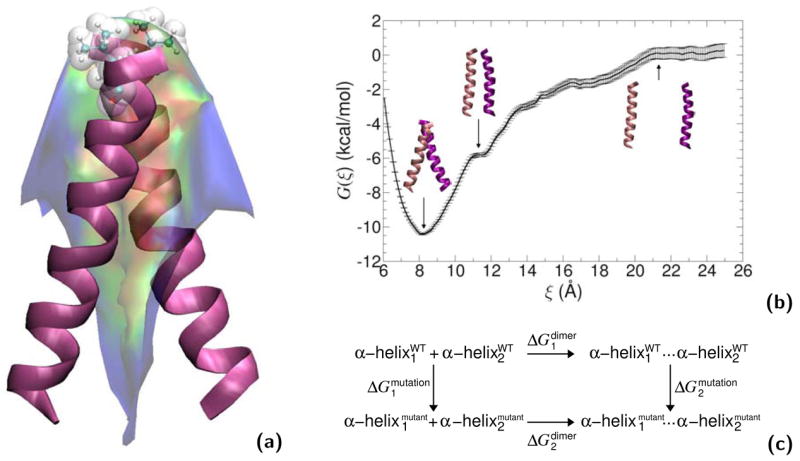
Homodimerization of the transmembrane (TM) domain of glycophorin A (GpA): (a): Contact surface of the two _α_-helices forming the TM domain of GpA. The strongest contacts are observed in the heptad of amino acids, Leu75, Ile76, Gly79, Val80, Gly83, Val84 and Thr87. Residue Leu75, which participates in the association of the two _α_-helices through dispersive interactions, is featured as transparent van der Waals spheres. (b): Free energy profile delineating the reversible dissociation of the two _α_-helices, obtained using an adaptive biasing force. The ordering parameter, ξ, corresponds to the distance separating the center of mass of the TM segments. The entire pathway was broken down into ten windows, in which up to 15 ns of MD sampling was performed, corresponding to a total simulation time of 125 ns. (c): Thermodynamic cycle utilized to perform the “alchemical transformation” of residues Leu75 and Ile76 into alanine, demonstrating the participation of these amino acids in the homodimerization of the two _α_-helices. The left vertical leg of the cycle represents the transformation in a single _α_-helix from the wild-type (WT) to the mutant form. The right vertical leg denotes a simultaneous point mutation in the two interacting _α_-helices. Using the notation of the figure, the free energy difference arising from this perturbation is equal to ΔG2mutation−2ΔG1mutation. Each leg of the thermodynamic cycle consists of 50 intermediate states and a total MD sampling of 6 ns. For clarity, the environment of the _α_-helical dimer, formed by a dodecane slab in equilibrium between two lamellae of water, is not shown.
Overcoming free energy barriers using an adaptive biasing force
The sizeable number of degrees of freedom described explicitly in statistical simulations of large molecular assemblies, in particular those of both chemical and biological interest, rationalizes the need for a compact description of thermodynamic properties. Free energy profiles offer a suitable framework that fulfills this requirement by providing the evolution of the free energy for chosen degrees of freedom. Determination of such free energy profiles, under the sine qua non condition that some ordering parameter, possibly a reaction coordinate, can be defined, however, remains a daunting task from the perspective of numerical simulations. In the context of Boltzmann sampling of the phase space, overcoming the high free energy barriers that separate thermodynamic states of interest is a rare event that is unlikely to occur on the timescales amenable to MD simulation.
An important step forward on the road towards an optimal sampling of the phase space along a chosen ordering parameter, ξ, has been made recently. In a nutshell, this new method relies on the continuous application of a dynamically adapted biasing force that compensates the current estimate of the free energy, thus virtually erasing the roughness of the free energy landscape as the system progresses along ξ [92]. To reach this goal, the average force acting on ξ, 〈Fξ_〉_ξ, is evaluated from an unconstrained MD simulation [93]:
| dA(ξ)dξ=〈∂U(r→1,…,r→N)∂ξ−1β∂ln∣J∣∂ξ〉ξ=−〈Fξ〉ξ | (29) |
|---|
where |J| denotes the determinant of the Jacobian for the transformation from Cartesian to generalized coordinates, which is a necessary modification of metric, given that {_r⃗_1, …, r⃗N} and ξ are not independent variables. The specific form of |J| is an inherent function of the ordering parameter, ξ, chosen to advance the system.
In the course of the simulation in NAMD, the force, Fξ, acting along the ordering parameter, ξ, is accrued in small bins, thereby supplying an estimate of the derivative d_A_(ξ)/d_ξ_. The adaptive biasing force (ABF), F⃗_ABF = − 〈 Fξ 〉_ξ ∇⃗rξ, is determined in such a way that, when applied to the system, it yields a Hamiltonian in which no average force is exerted along. As a result, all values of ξ are sampled with an equal probability, which, in turn, dramatically improves the accuracy of the calculated free energies. It further entails that progression of the system along ξ is fully reversible and limited solely by its self-diffusion properties. At this stage, it should be clearly understood that whereas the ABF method enhances sampling along the ordering parameter, ξ, its ability to supply a perfectly uniform probability distribution of the system over the entire range of ξ values may be impeded by possible orthogonal degrees of freedom in the slow manifolds.
It has been chosen to introduce the average force method in NAMD within the convenient framework of unconstrained MD [93], which should not be construed in such a way that none of the degrees of freedom of the system can be frozen in time. It merely indicates that the ordering parameter, ξ, is unconstrained. Either constraint forces must be taken into account in Fξ, as they are in NAMD version 2.6, or it will be crucial to ascertain that no Cartesian coordinate appears simultaneously in a constrained degree of freedom and in the derivative ∂U(_r⃗_1, …, r⃗N)/∂ξ of equation (29).
The ABF scheme available in NAMD features different reaction coordinates that may be applied to a host of problems of both chemical and biophysical relevances. This includes, among others, the intramolecular folding of a short peptide, the partitioning of small solutes across an aqueous interface and the intermolecular association of neutral and ionic species [92, 93].
The _α_-helical dimerization of GpA represents an interesting application of the method, whereby the reversible dissociation—rather than the association, for obvious cost-effectiveness reasons—is carried out, using the distance separating the center of mass of the TM segments as the reaction coordinate. The free energy profile characterizing this process is shown in Figure 8 and features a deep minimum at ca. 8.2 Å, which corresponds to the native, close packing of the _α_-helices.
As the TM segments move away from each other, helix-helix interactions are progressively disrupted, in particular in the crossing region, thus, causing an abrupt increase of the free energy, accompanied by a tilt of the two _α_-helices towards an upright orientation. As the distance between the two TM segments further increases, the free energy profile levels off at ca. 21 Å, a separation beyond which the dimer is fully dissociated.
A valuable feature offered by NAMD lies in the possibility to evaluate a posteriori electrostatic and van der Waals forces from an ensemble of configurations. Projection of these forces onto the reaction coordinate, ξ, and subsequent integration of the former provides a deconvolution of the complete free energy profile in terms of helix-helix and helix-solvent contributions.
Analysis of these contributions reveals two regimes in the association process, driven at large separation by the solvent, which pushes the _α_-helices together, and at short separation by van der Waals interactions that favor native contacts [96].
3 NAMD software design
Just as the intelligent car buyer looks under the hood to understand the performance and longevity of a particular vehicle, we now direct the attention of the reader and potential NAMD user to a few design and implementation details that contribute to the flexibility and performance of NAMD.
3.1 Goals, design, and implementation
NAMD was developed to enable ambitious MD simulations of biomolecular systems, employing the best technology available to provide the maximum performance possible to researchers. In the past decade simulation size and duration have increased dramatically. Ten years ago a simulation of 36,000 atoms over 100 ps as reported in [5] was considered very advanced. Today this status is reserved for simulations of systems with more than 300,000 atoms for up to 100 ns as reported in [6, 23, 55]. The progress made is illustrated in Fig. 1, comparing the sizes of systems reported in [5] and [6]. This thousand-fold increase in capability (ten-fold in atom count and over hundred-fold in simulation length) has been partially enabled by advances in processor performance, with clock rate increases leading the way. However, substantial progress has also resulted from exploiting the factor of one hundred or more in performance available through the use of massively parallel computing, coordinating the efforts of numerous processors to address a single computation.
Looking forward, scientific ambition remains unchecked while increases in processor clock rates are constrained by limits on power consumption and heat dissipation. This stagnation in CPU speed has inspired system vendors such as Cray and SGI to incorporate field-programmable gate arrays (FPGAs) into their offerings, promising great performance increases, but only for suitable algorithms that are subjected to heroic porting efforts (as have been initiated for the force evaluations used by NAMD). Advances in semiconductor technology will surpass the limits encountered today, but in the meantime industry has turned to offering greater concurrency to performance-hungry applications, scaling systems to more processors, and processors to more cores, rather than to higher clock rates. Indeed, the highest-performance component of a modern desktop is often the 3D graphics accelerator, which inexpensively provides an order of magnitude greater floating point capability than the main processor at a fraction of the clock rate by automatically distributing independent calculations to tens of pipelines, and even across multiple boards. Therefore, high performance and parallel computing will become even more synonymous than today, with greater industry acceptance and support.
Scientific computing is also facing the perennial “software crisis” that has stalked business information systems for decades. The seminal Allen and Tildesley [97] could dedicate a few pages of an appendix to writing efficient FORTRAN-77 code and consider the reader well-informed. Developing modern high-performance software, however, requires knowledge of everything from parallel decomposition and coordination libraries to the relative cost of accessing different levels of cache memory. The design of more complex algorithms and numerical methods has ensured that any useful and successful program is likely to outlive the machine for which it is originally written, making portability a necessity. Software is also likely to be used and extended by persons other than the original author, making code readability and modifiability vital.
Software maintenance activities such as porting and modification account for the majority of the cost and effort associated with a program during its lifetime. These issues have been addressed in the development of object-oriented software design, in which the programmer breaks the program into “objects” comprising closely-related data (such as the x, y, and z components of a vector) and the operations that act on it (addition, dot product, cross product, etc.). The objects may be arranged into hierarchies of classes, and an object may contain or refer to other objects of the same or different classes. In this manner, large and complex programs can be broken down into smaller components with defined interfaces that can be implemented independently. NAMD is implemented in C++, the most popular and widely supported programming language providing efficient support for these methods.
Methodology for the development of parallel programs is far from mature, with automatically parallelizing compilers and languages still quite limited and most programmers using the Message Passing Interface (MPI) libraries in combination with C, C++, or Fortran. While the acceptance of MPI as a cross-platform standard for parallel software has been of great benefit, the burden on the programmer remains. The first task is to decompose the problem, which is often simplified by assuming that the processor count is a power of two or has factors corresponding to the dimensions of a large three-dimensional array. MPI programming then requires the explicit sending and receiving of arrays between processors, much like directing a large and complex game of catch.
NAMD is based on the Charm++ parallel programming system and runtime library [98]. In Charm++, the computation is decomposed into objects that interact by sending messages to other objects on either the same or remote processors. These messages are asynchronous and one-sided, i.e., a particular method is invoked on an object whenever a message arrives for it rather than having the object waste resources while waiting for incoming data. This message-driven object programming style effectively hides communication latency and is naturally tolerant of the system noise that is found on workstation clusters. Charm++ also supports processor virtualization [99], allowing each algorithm to be written for an ideal, maximum number of parallel objects that are then dynamically distributed among the actual number of processors on which the program is run. Charm++ provides these benefits even when it is implemented on top of MPI, an option that allows NAMD to be easily ported to new platforms.
The parallel decomposition strategy used by NAMD is to treat the simulation cell (the volume of space containing the atoms) as a three-dimensional patchwork quilt, with each patch of sufficient size that only the 26 nearest neighboring patches are involved in bonded, van der Waals, and short-range electrostatic interactions. More precisely, the patches fill the simulation space in a regular grid and atoms in any pair of non-neighboring patches are separated by at least the cutoff distance at all times during the simulation. Each hydrogen atom is stored on the same patch as the atom to which it is bonded, and atoms are reassigned to patches at regular intervals. The number of patches varies from one to several hundred and is determined by the size of the simulation independently of the number of processors.
When NAMD is run, patches are distributed as evenly as possible, keeping nearby patches on the same processor when there are more patches than processors, or spreading them across the machine when there are not. Then, a (roughly 14 times) larger number of compute objects responsible for calculating atomic interactions either within a single patch or between neighboring patches is distributed across the processors, minimizing communication by grouping compute objects responsible for the same patch together on the same processors. At the beginning of the simulation, the actual processor time consumed by each compute object is measured and this data is used to redistribute compute objects to balance the workload between processors. This measurement-based load balancing [100] contributes greatly to the parallel efficiency of NAMD.
Using forces calculated by the compute objects, each patch is responsible for integrating the equations of motion for the atoms it contains. This can be done independently of other patches, but occasionally requires global data affecting all atoms, such as a change in the size of the periodic cell due to a constant pressure algorithm. While the integration algorithm is the clearly visible “outer loop” in a serial program, NAMD’s message-driven design could have resulted in much obfuscation (as was experienced even in the simpler NAMD 1.X [4]). This was averted by using Charm++ threads to write a top-level function that is called once for each patch at program start and does not complete until the end of the simulation [101]. This design has allowed pressure and temperature control methods and even a conjugate gradient minimizer to be implemented in NAMD without writing any new code for parallel communication.
3.2 Tcl scripting interface
NAMD has been designed to be extensible by the end user in those areas that have required the most modification in the past and that are least likely to affect performance or harbor hard-to-detect programming errors. The critical force evaluation and integration routines that are the core of any molecular dynamics simulation have remained consistent in implementation as NAMD has evolved, occasionally introducing improved methods for pressure and temperature control. The greatest demand for modification has been in high-level protocols, such as equilibration and simulated annealing schedules. An additional demand has been for the implementation of experimental and often highly specialized steering and analysis methods, such as used to study the rotational motion of ATP synthase [85].
Flexibility requirements could in theory be met by having the end user modify NAMD’s C++ source code, but this is undesirable for several reasons. Any users with special needs would have to maintain their own “hacked” version of the source code, which would need to be updated whenever a new version of NAMD was released. These unfortunate users would also need to maintain a full compiler environment and any external libraries for every platform on which they wanted to run NAMD. Finally, an understanding of both C++ and NAMD’s internal structure would be required for any modification, and bugs introduced by the end user would be difficult for a novice programmer to fix. These problems can be eliminated by providing a scripting interface which is interpreted at run time by NAMD binaries that can be compiled once for each platform and installed centrally for all users on a machine.
Tcl (Tool Command Language) [102] is a popular interpreted language intended to provide a ready-made scripting interface to high performance code written in a “systems programming language” such as C or C++. The Tcl programmer is supported by online documentation (at www.tcl.tk) and by books targeting all levels of experience. Tcl is used extensively in the popular molecular graphics program VMD, and therefore even novice users are likely to have experience with the language. In NAMD, Tcl is used to parse the simulation configuration file, allowing variables and expressions to be used in initially defining options, and then to change certain options during a running simulation.
Tcl scripting has been used to implement the replica exchange method [103] using NAMD, without modifying or adding a single line of C++. A master program, running in a Tcl shell outside of NAMD, is used to spawn a separate NAMD slave process for each replica needed. Each NAMD instance is started with a special configuration file that uses the standard networking capabilities of Tcl to connect to the master program via a TCP socket. At this point, the master program sends commands to each slave to load a molecule, simulate dynamics for a few hundred steps, report average energies, and change temperatures based on the relative temperatures of the other replicas. This work would have been much more difficult without a standard and fully featured scripting language such as Tcl.
NAMD provides a variety of standard steering forces and protocols, but an additional Tcl force interface provides the ultimate in flexibility. The user specifies the atoms to which steering forces will be applied; the coordinates of these atoms are then passed to a Tcl procedure, also provided by the user, at every timestep. The Tcl steering procedure may use these atomic coordinates to calculate steering forces, possibly modifying them based on elapsed time or progress of the atoms along a chosen path. This minimal but complete interface has been used to implement complex features such as the adaptive biasing force method [93] of Sec. 2.6.
3.3 Serial and parallel performance
While the NAMD developers have strived to make the software as fast as possible [104], decisions made by the user can greatly influence the serial performance and parallel efficiency of a particular simulation. For example, the computational effort required for a simulation is dominated by the nonbonded force evaluation, which scales as NRcut3ρ where N is the number of simulated atoms, Rcut is the cutoff distance, and ρ = N/V is the number of atoms per unit volume. From this formula one can see that, e.g., a 5-point water model compared to a 3-point water model increases both the number and density of simulated points (real and dummy atoms) and would therefore run up to (5/3)2 = 2.8 times as long.
The processor type and clock rate of the machine on which NAMD is run, of course, will affect performance. Unlike many scientific codes, NAMD is usually limited by processor speed rather than memory size, bandwidth, or latency; the patch structure described above leads to naturally cache-friendly data layout and force routines. However, the nonbonded pair lists used by NAMD, while distributed across nodes in a parallel run, can result in paging to disk for large simulations on small memory machines, e.g., 100,000 atoms on a single 128 MB workstation; in this case disabling pair lists will greatly improve performance.
The limits of NAMD’s parallel scalability are mainly determined by atom count, with one processor per 1000 atoms being a conservative estimate for good efficiency on recent platforms. Increased cutoff distances will result in additional work to distribute, but also in fewer patches, and hence one is confronted with a hard-to-predict effect on scaling. Finally, dynamics features that require global communication or even synchronization, such as minimization, constant pressure, or steering, may adversely affect parallel efficiency.
When procuring a parallel computer, great attention is normally paid to individual node performance, network bandwidth, and network latency. While NAMD transfers relatively little data and is designed to be latency tolerant, scaling beyond a few tens of processors will benefit from the use of more expensive technologies than commodity gigabit ethernet. A major drain on parallel performance will come from interference by other processes running on the machine. A cluster should never be time-shared, with two parallel jobs running on the same nodes at the same time, and care should be taken to ensure that orphaned processes from previous runs do not remain. On larger machines, even occasional interruptions for normal operating system functions have been shown to degrade the performance of tightly coordinated parallel applications running on hundreds of processors [105].
The particle mesh Ewald (PME) method for full electrostatics evaluation, neglected in the performance discussion thus far, deserves special attention. The most expensive parts of the PME calculation are the gridding of each atomic charge onto (typically) 4 × 4 × 4 points of a regular mesh and the corresponding extraction of atomic forces from the grid; both scale linearly with atom count. The actual calculation of the (approximately) 100 × 100 × 100 element fast Fourier transform (FFT) is negligible, but requires many messages for its parallel implementation. While this presents a serious impediment to other programs, NAMD’s message-driven architecture is able to automatically interleave the latency-sensitive FFT algorithm with the dominant and latency-tolerant short-range nonbonded calculation [106]. In conclusion, a simulation with PME will run slightly slower than a non-PME simulation using the same cutoff, but PME is the clear winner because it provides physically correct electrostatics (without artifacts due to truncation) and allows a smaller short-range cutoff to be used.
When running on a parallel computer, it is important to measure the parallel efficiency of NAMD for the specific combination of hardware, molecular system, and algorithms of interest. This is correctly done by measuring the asymptotic cost of the simulation, i.e., the additional runtime of a 2000 step run versus a 1000 step run, thereby discounting startup and shutdown times. By measuring performance at a variety of processor counts, a decision can be made between, e.g., running two jobs on 64 procesors each versus one job 60% faster (and 20% less efficiently) on 128 processors.
Dynamic load balancing makes NAMD’s startup sequence longer than that of other parallel programs, requiring special attention to benchmarking. Initial load balancing in a NAMD run begins by default after five atom migration “cycles” of simulation. Compute object execution times are measured for five cycles, followed by a major load balancing in which work is reassigned to processors from scratch. Next is five cycles of measurement followed by a load balance refinement in which only minor changes are attempted. This is repeated immediately, and then periodically between 200-cycle stretches of simulation with measurement disabled (for maximum performance). After the second refinement, NAMD will print several explicitly labeled “benchmark” timings, which are a good estimate of performance for a long production simulation. The results of such benchmarking on a variety of platforms for a typical simulation are presented in Fig. 9.
Figure 9.
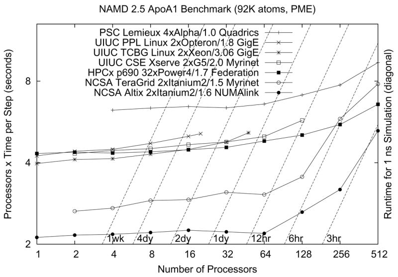
NAMD performance on modern platforms. The cost in CPU seconds of a single timestep for a representative system of 92,000 atoms with a 12 Å short-range cutoff and full electrostatics evaluated via PME every four steps is plotted on the vertical axis, while the wait for a 1 ns simulation (one million timesteps of 1 fs each) may be read relative to the broken diagonal lines. Perfect parallel scaling is a horizontal line. The older PSC Lemieux Alpha cluster has lower serial performance but scales very well. The HPCx IBM POWER 4 cluster at Edinburgh scales similarly, with comparable serial performance to the Xeon, Opteron, and Apple Xserve G5 clusters at Urbana. The two NCSA Itanium platforms have excellent serial performance but lose efficiency beyond 128 processors.
While every researcher’s situation is different, the computational resource decisions made by the authors’ group provide a useful example. The main local resources are six independent, 24-node, 48-processor Linux clusters using commodity gigabit ethernet cards and switches. Each cluster is used for at most one simulation at a time, and therefore only the six head nodes are connected to the building network, which provides access to central file and administrative servers. A queueing system manages a single queue, dispatching jobs in order to the next free cluster for up to 24 hours, yielding full utilization as long as jobs are available to run. In addition, the Clustermatic Linux distribution allows a running simulation to be easily suspended by the queueing system, allowing short “express” jobs to run, which are used for simulation setup and testing, as well as for on-demand IMD. These cost-efficient local resources are supplemented by grants of computer time from NSF-funded centers, which provide access to larger, more scalable machines for large, intensive simulations and other special cases.
In conclusion, a basic understanding of NAMD’s performance characteristics combined with specific benchmarks provides more science in less time. Conversely, the most common ways to waste computer time with NAMD are to include too much water in the simulation cell, to use an unnecessarily large cutoff with PME, to run on more processors than the simulation efficiently scales to, to blindly continue a simulation without checking the output for anomalies, and, finally, to simulate a molecule without a clear understanding of what scientific questions are to be answered based on the results.
4 Three exemplary applications
In the following we describe three exemplary applications of NAMD. The applications are chosen to illustrate the use of NAMD in studies of small (ubiquitin), intermediate (aquaporin channel), and large (lac repressor) systems. We emphasize in particular the features of NAMD which were most useful and how they allowed us to surmount methodological hurdles quickly.
4.1 Ubiquitin
Our first application of the NAMD program involves a rather routine modeling project on a small protein system that grew into a more extensive one over time. The reader will learn from this first brief case study mainly how NAMD is used under common circumstances in which any other modeling program would have performed just as well, though we will emphasize the particular features that made NAMD a very suitable choice. The protein investigated is ubiquitin, which recently acquired considerable notice as the main subject of study by the 2004 Nobel laureates in Chemistry [107, 108]. Ubiquitin is a small globular protein of about eighty amino acids that is highly conserved throughout the eukaryotes. The proteins, usually in the form of multimers, function as tags for the destination of cellular proteins in cell traffcking, e.g., for protein degradation [109]. The modeling task in the present case was to explain atomic force microscopy experiments that measured forces and extensions that arise when monomeric or tetrameric ubiquitin is stretched with pN forces [110, 111]. The project was vastly simplified through the availability of tutorials that explained how VMD and NAMD are used to set up a simulation of the solvated protein, to stretch it, and to analyze the results (http://www.ks.uiuc.edu/Training/Tutorials). Indeed, VMD and NAMD are accessible to novice researchers due to the extensive introductory material prepared by the developers.
The goal of these simulations was to stretch monomeric ubiquitin using the steered molecular dynamics method introduced above. After equilibration of the protein in a spherical water bath (a system of altogether 26,000 atoms) under NVT and NVE ensemble conditions with a 12 Å cutoff of nonbonded forces, the protein was stretched with the N-terminus constrained and the C-terminus pulled with a spring (spring constant of about 500 pN/Å mol), the end of which moved at a speed of 0.5 Å/ps (c.f., Eq. (17) and Fig. 6). Snapshots during the stretching process are shown in Fig. 10. One can recognize that the protein can be stretched readily from the folded to the completely extended conformation. The simulations lasted about a nanosecond and, with a 2 fs timestep, required four days on a desktop computer with an AMD Opteron processor.
Figure 10.
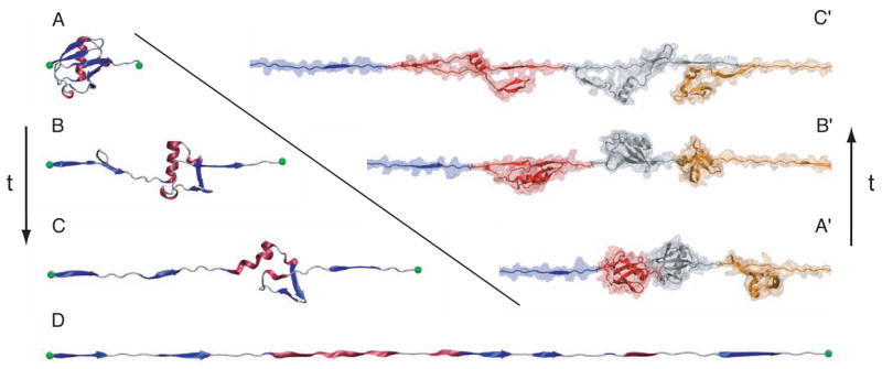
Pulling ubiquitin and tetra-ubiquitin. (A)–(D) mono-ubiquitin is shown at various stages of a constant velocity SMD simulation with the N and C termini highlighted in green. The different structures are seen to unfold at different moments in the simulation. (A′)–(C′) tetra-ubiquitin is shown being pulled with constant force. Each color represents a different monomer and the transparent portion is the surface of the protein with the first and fourth segments not completely shown. Again, the different subunits can be seen to come apart at different times.
Next, the stretching of a tandem of four ubiquitins was also attempted. In this case, the simulated protein-water system comprised 62,000 atoms; snapshots during the 3.5 ns stretching process are also shown in Fig. 10. The simulations revealed the unfolding pathways of stretched ubiquitin, information that cannot be gleaned from an experiment that provides solely data of extension and applied forces vs. time. This application of steered molecular dynamics demonstrates well the value of molecular modeling in complementing experimental observation. The ready accessibility and ease of use of NAMD makes such modeling projects possible for experimentalists.
In this project several key features of NAMD and VMD were employed. NAMD ran on a common desktop system and was even used on a laptop, e.g., for setting up and testing the simulation. NAMD simulations can then easily be migrated to multi-processor machines, though in the present case that was not absolutely necessary. The “Psfgen” plugin of VMD was very useful in setting up the system, namely in defining the chemical topology, i.e., the LYS48-C-terminus bonds connecting the four tandem repeats, and generating so-called protein structure and parameter files. Also beneficial was the “Solvate” plugin of VMD, which greatly expedited the task of placing ubiquitin in a water bath. NAMD is ideally suited to carry out SMD simulations; as explained above, the needed functionality can be activated at the input file level and other features can be added through scripting. In the present case, the scripting capabilities of VMD allowed us to calculate the extension of the protein reached at any moment during the stretching process. This easy provision of all types of data from an MD run as well as the interplay with VMD are invaluable features of NAMD.
4.2 Aquaporin
The second example of using NAMD to simulate and investigate a biomolecular process concerns a family of membrane proteins, known as aquaporins (AQPs), which are responsible for facilitating water transfer across cellular membranes. Simulation of the dynamics and function of these channels is a good example of systems that require inclusion of more than 100,000 atoms in the molecular system [112, 113, 114, 115], as one needs to explicitly include a lipid bilayer and water in order to provide a natural environment to the protein and to be able to investigate transmembrane diffusion of molecules. Conceptual and methodological issues of simulating membrane proteins have been reviewed in [116, 117]. The size of the system and the computational demand are usually prohibitive factors in simulation studies of membrane proteins, but NAMD’s ability to exploit efficiently hundreds of processors makes it possible to tackle such problems with full atomic detail in the most faithful way possible. A side view of an AQP model embedded in a lipid bilayer is shown in Fig. 11. AQPs are passive membrane channels that increase (over that of pure membranes) the rate of water exchange between the cell and its environment in a highly selective manner. Some members of the family have dual functions in cellular metabolism, as they also allow other small molecules, such as glycerol, to pass. Charged species, including protons, however, are excluded.
Figure 11.
Side view of a simulated aquaporin tetramer in the cell membrane. The E. coli water/glycerol channel GlpF is embedded in a patch of POPE lipid bilayer and fully hydrated by water on both sides. Lipid head groups are shown in CPK and the hydrophobic tail region is drawn using licorice representation. The four AQP monomers, each forming an independent water pore, are shown in different colors. The single file of water formed inside the pores is shown in one of the monomers. The characteristic conformational inversion of water at the center of the channel that contributes to the barrier against proton transfer is discernible.
Simulation of water permeation through AQPs and the study of selectivity mechanisms employed by the channel require simulations of large molecular aggregates on the order of several tens of nanoseconds [114, 115, 118, 58]. NAMD proved to be very efficient in simulating such systems at ambient pressure and physiological temperature with full account of electrostatic forces. These conditions are critical for a reliable description of the molecular system at hand. NAMD provides a variety of pressure control schemes that are effective and useful in the initial setup and equilibration phases of simulations. For example, NAMD allows exclusion of atoms from pressure calculation, which enables one to fix the protein during the initial simulation of its environment under constant-pressure conditions. Multi-nanosecond equilibrium simulations performed by NAMD successfully described diffusive permeation of water through the channel, in close agreement with the natural time scale (nanoseconds) of the event [114, 118]. A key finding of the simulations was a unique configuration of water enforced by the channel during the permeation. This configuration was found to be an effective, novel selection mechanism that prevents proton transfer in these channels [114, 118]. In order to investigate the permeation of larger substrates, i.e., glycerol and longer linear sugar molecules, we took advantage of the SMD and IMD methodologies that are easily accessible through NAMD. SMD simulations of glycerol permeation through GlpF allowed us to reconstruct the potential of mean force of the process [62]. IMD simulations that permit one to rapidly sample various configurations of a complex between a macromolecule and small molecules were applied to study how sugar molecules interact with the narrowest part of the channel, the selectivity filter, and how these interactions furnish the stereoselectivity of the channel [53].
The Tcl scripting capability of NAMD and its atom selection algorithms allowed us to apply external forces of different magnitude and direction to dynamically changing groups of water molecules and, thereby, generate hydrostatic pressure gradients across the membrane of interest [115, 58, 119]. Applying this method, and taking advantage of the speed of the simulations provided by NAMD and its high performance on various platforms (Fig. 9), we were able to calculate the water permeation rate through the channel using several simulations performed at various hydrostatic pressure gradients in either direction, and determine the osmotic permeability of AQPs, a property that can be directly compared to experimentally measured values for these channels [115, 58, 119]. In these simulations external forces were applied to a large group of molecules (water molecules in the bulk) whose number and positions are constantly changing as the simulations proceed. The modularity of the NAMD code allowed us to easily add the force application part of the calculations into the code, thus avoiding any compromise in the performance and scalability of the program. A very important advantage of NAMD in this respect is that the user does not need to know parallel programming in order to implement new features and add modules to the program.
4.3 Multiscale lac repressor – DNA complex
Our third example for the use of NAMD concerns a protein-DNA complex involving the lac repressor (LacI) that is a paradigm for gene control. We choose this example since it leads to a simulation of very large size (310,000 atoms) that also requires great flexibility in the simulation protocol in combining all-atom molecular dynamics with continuum mechanics.
LacI regulates the function of the lac operon, a set of genes responsible for lactose digestion in Escherichia coli; when lactose is not present as a metabolite in the environment, LacI inhibits the expression of these genes by binding to two nearby sites at the beginning of the operon and folding the intervening DNA into a loop. The detailed mechanics of the LacI-DNA interaction remain unknown even though the crystallographic structure of LacI bound to its cognate DNA segments is available [120, 121] along with extensive biochemical and genetic data [122, 123]. In particular, the structure in [120] does not include the DNA loop connecting the two bound DNA segments nor does it provide information on how LacI wrestles the DNA, forcing it to maintain a loop form.
A key obstacle to the simulation of the LacI-DNA dynamics is that LacI alone is a very large protein that results, together with a water bath, in a system of 300,000 atoms; including the DNA loop would increase the size to 700,000 atoms thus incurring an even greater computational cost. To overcome this difficulty one can follow a multiscale strategy and describe the DNA loop mathematically employing the Kirchhoff theory of continuum elastic rods as developed in [124], coupling the calculation to an all-atom MD representation of LacI. The method has been outlined in [86] and applied in [6]. The lacI-DNA structure constructed in [125] and employed in [6] is available in the Protein Data Bank (1Z04) [126]. In the simulation, illustrated in Fig. 12, LacI was solvated in a box of TIP3P water and 100 mM NaCl and simulated under NPT ensemble conditions with periodic boundary conditions and PME electrostatics for an overall simulation time of 40 ns using a 1 fs time step. At 10 ps intervals, position and orientation of the LacI head groups were communicated to the mathematical description of the DNA loop, which determined the appropriate new loop geometry and communicated back the forces and torques with which the DNA resisted the protein’s action; forces and torques were included in the MD simulations much like forces are incorporated in SMD runs. Simulation results are shown in Fig. 12. One can recognize the large scale motion of the DNA loop over the course of the simulation. A key finding resulting from the simulation is an extreme flexibility of the two LacI head groups absorbing most of the strain arising from the DNA loop. The simulations reported in [6] provided also an insightful new interpretation of prior FRET data [127].
Figure 12.
Snapshots taken over the course of the LacI-DNA complex multiscale simulation: (a) The evolution of the structure of the DNA loop; (b) The structure of LacI remains unchanged, with the exception of the rotation of the head groups, which allows the DNA loop to adopt a more relaxed configuration.
NAMD proved to be most valuable due to its ability to efficiently simulate very large systems. In the present case NAMD ran a 310,000 atom system on 256 Itanium processors of the NCSA TeraGrid system with an average production speed of 2.5 ns per day. The multiscale strategy linking MD with a continuum mechanics DNA model was implemented through the Tcl scripting interface of NAMD. This feature permitted us not only to obtain information from the simulation, e.g., head group geometries, on the fly, but also to control from the NAMD side the calculations for the DNA model, eventually retrieving the forces applied in the LacI simulation. For the sake of clarity we emphasize that the entire multiscale simulation, including the continuum mechanics description of DNA, was controlled from the NAMD program and its Tcl scripting feature. Since NAMD readily permits the definition of all types of external forces, the implementation of the multiscale strategy was straightforward. We note here also that the ability of NAMD to write and read any type of files during its execution proved to be invaluable for the ultimate analysis of the multiscale simulation data.
5 Conclusion
We conclude our overview of NAMD with a list of the program’s key features in Table 1. Surveys indicate consistently that users greatly appreciate that NAMD is distributed free of charge. NAMD is well known for its performance on large parallel computers, for which it has received a Gordon Bell award [106], but the program is actually used on many platforms, including laptops. This versatility is a great benefit for initiating and testing modeling projects. NAMD permits a novice to carry out standard simulations of most types readily, but NAMD also supports more advanced uses. The most essential feature in this regard is NAMD’s Tcl scripting capability, which has been used to implement, e.g., replica exchange dynamics, adaptive biasing forces, and advanced phase space sampling protocols.
NAMD is complemented by the molecular graphics program VMD to offer a complete modeling environment. In addition to its other functions, VMD provides tools tailored to NAMD. This is a natural development since not only do the programs share a large common user base, but they are also being developed together and use the same scripting language. VMD provides assistance at all stages of a simulation including preparing the initial system, monitoring the progress of the calculation, and analyzing the results. Initiating a modeling project is simplified and accelerated through convenient features that aid in the typical tasks of building a model, e.g., solvating a protein or placing it in a lipid bilayer, and providing the needed protein structure files. VMD’s AutoIMD feature allows one to modify and/or interact with the system “on the fly” with both immediate visual and mechanical feedback, thus providing an intuitive method of exploring the system in ways not available through scripting alone. Finally, VMD provides a unique analysis environment for the results of NAMD simulations. For example, one can use VMD for routine calculations such as protein stability or intra- and intermolecular distances, as well as advanced ones such as electrostatic potential maps. Furthermore, the analysis capabilities of VMD may be extended through Tcl scripting, allowing the user to design any project-specific tools needed. Clearly, although NAMD and VMD function effectively as stand-alone programs, their highest purpose is achieved when used together.
NAMD users also benefit from the program BioCoRE [128], a web-based collaborative research environment that is linked to both NAMD and VMD. For example, BioCoRE greatly simplifies submission of NAMD simulations to supercomputer centers and local machines alike. BioCoRE also provides a graphical user interface to prepare simulation input files.
The authors’ group focuses much effort on training researchers in the use of NAMD through a series of tutorials available on the web. The NAMD web site is a continuously updated source of information for novice and advanced users (http://www.ks.uiuc.edu/Research/namd/).
Acknowledgments
The NAMD source code has been written, revised, and extended by many talented individuals, including (in alphabetical order) Milind Bhandarkar, Robert Brunner, Christophe Chipot, Andrew Dalke, Surjit Dixit, Paul Grayson, Justin Gullingsrud, Attila Gursoy, David Hardy, Jérôme Hénin, Bill Humphrey, David Hurwitz, Neal Krawetz, Sameer Kumar, David Kunzman, Chee Wai Lee, Mark Nelson, James Phillips, Aritomo Shinozaki, Gengbin Zheng, Fangqiang Zhu, and most certainly others for whose omission from this list we apologize. The authors would also like to acknowledge Fatemeh Khalili-Araghi and Marcos Sotomayor for preparing the ubiquitin tetramer and ubiquitin simulations.
Funding for the Resource for Macromolecular Modeling and Bioinformatics is provided by the National Institutes of Health grant NIH P41 RR05969. Free energy calculation development with C. Chipot was aided by a CNRS/UIUC collaborative grant. The authors gladly acknowledge supercomputer time provided by the Pittsburgh Supercomputer Center and the National Center for Supercomputing Applications via National Resources Allocation Committee grant MCA93S028.
References
- 1.Kalé Laxmikant, Skeel Robert, Bhandarkar Milind, Brunner Robert, Gursoy Attila, Krawetz Neal, Phillips James, Shinozaki Aritomo, Varadarajan Krishnan, Schulten Klaus. NAMD2: Greater scalability for parallel molecular dynamics. J Comp Phys. 1999;151:283–312. [Google Scholar]
- 2.Humphrey William, Dalke Andrew, Schulten Klaus. VMD – Visual Molecular Dynamics. J Mol Graphics. 1996;14:33–38. doi: 10.1016/0263-7855(96)00018-5. [DOI] [PubMed] [Google Scholar]
- 3.Nelson Mark, Humphrey William, Gursoy Attila, Dalke Andrew, Kalé Laxmikant, Skeel Robert, Schulten Klaus, Kufrin Richard. MDScope – A visual computing environment for structural biology. Comput Phys Commun. 1995;91(1–3):111–134. [Google Scholar]
- 4.Nelson Mark, Humphrey William, Gursoy Attila, Dalke Andrew, Kalé Laxmikant, Skeel Robert D, Schulten Klaus. NAMD – A parallel, object-oriented molecular dynamics program. Int J Supercomp Appl High Perform Comp. 1996;10:251–268. [Google Scholar]
- 5.Kosztin Dorina, Bishop Thomas C, Schulten Klaus. Binding of the estrogen receptor to DNA: The role of waters. Biophys J. 1997;73:557–570. doi: 10.1016/S0006-3495(97)78093-7. [DOI] [PMC free article] [PubMed] [Google Scholar]
- 6.Villa Elizabeth, Balaeff Alexander, Schulten Klaus. Structural dynamics of the Lac repressor-DNA complex revealed by a multiscale simulation. Proc Natl Acad Sci USA. 2005;102:6783–6788. doi: 10.1073/pnas.0409387102. [DOI] [PMC free article] [PubMed] [Google Scholar]
- 7.MacKerell AD, Jr, Bashford D, Bellott M, Dunbrack RL, Jr, Evanseck J, Field MJ, Fischer S, Gao J, Guo H, Ha S, Joseph D, Kuchnir L, Kuczera K, Lau FTK, Mattos C, Michnick S, Ngo T, Nguyen DT, Prodhom B, Reiher IWE, Roux B, Schlenkrich M, Smith J, Stote R, Straub J, Watanabe M, Wiorkiewicz-Kuczera J, Yin D, Karplus M. All-atom empirical potential for molecular modeling and dynamics studies of proteins. J Phys Chem B. 1998;102:3586–3616. doi: 10.1021/jp973084f. [DOI] [PubMed] [Google Scholar]
- 8.Weiner SP, Kollman PA, Case DA, Singh UC, Ghio C, Alagona G, Profeta J, Weiner P. A new force field for molecular mechanical simulation of nucleic acids and proteins. J Am Chem Soc. 1984;106:765–784. [Google Scholar]
- 9.Berendsen HJC, van der Spoel D, van Drunen R. GROMACS: A message passing parallel molecular dynamics implementation. Comput Phys Commun. 1995;91:43–56. [Google Scholar]
- 10.Weiner Paul K, Kollman Peter A. AMBER: Assisted model building with energy refinement. A general program for modeling molecules and their interactions. J Comp Chem. 1981;2(3):287–303. [Google Scholar]
- 11.Ewald P. Die Berechnung optischer und elektrostatischer Gitterpotentiale. Ann Phys. 1921;64:253–287. [Google Scholar]
- 12.de Leeuw SW, Perram JW, Smith ER. Simulation of electrostatic systems in periodic boundary conditions. I. Lattice sums and dielectric constants. Proc R Soc Lond A. 1980;373:27–56. [Google Scholar]
- 13.Grubmüller H, Heller H, Windemuth A, Schulten K. Generalized Verlet algorithm for efficient molecular dynamics simulations with long-range interactions. Molecular Simulation. 1991;6:121–142. [Google Scholar]
- 14.Loncharich Richard J, Brooks Bernhard R. The effects of truncating long-range forces on protein dynamics. Proteins: Stru Func and Genetics. 1989;6:32–45. doi: 10.1002/prot.340060104. [DOI] [PubMed] [Google Scholar]
- 15.Feller Scott E, Pastor Richard W, Rojnuckarin Atipat, Bogusz Stephen, Brooks Bernard R. Effect of electrostatic force truncation on interfacial and transport properties of water. J Phys Chem. 1996;100:17011–17020. [Google Scholar]
- 16.Bergdorf M, Peter C, Hünenberger PH. Influence of cut-off truncation and artificial periodicity of electrostatic interactions in molecular simulations of solvated ions: A continuum electrostatics study. J Chem Phys. 2003;119:9129–9144. [Google Scholar]
- 17.Kastenholz MA, Hünenberger PH. Influence of artificial periodicity and ionic strength in molecular dynamics simulations of charged biomolecules employing lattice-sum methods. J Phys Chem B. 2004;108:774–788. [Google Scholar]
- 18.Weber W, Hünenberger PH, McCammon JA. Molecular dynamics simulations of a polyalanine octapeptide under Ewald boundary conditions: Influence on artificial periodicity of peptide conformation. J Phys Chem B. 2000;104:3668–3675. [Google Scholar]
- 19.Perram JW, Petersen HG, de Leeuw SW. An algorithm for the simulation of condensed matter which grows as the 3/2 power of the number of particles. Mol Phys. 1988;65:875–889. [Google Scholar]
- 20.Darden Tom A, York Darrin M, Pedersen Lee G. Particle mesh Ewald: An Nlog(N) method for Ewald sums in large systems. J Chem Phys. 1993 November 15;98(10):10089. [Google Scholar]
- 21.Essmann U, Perera L, Berkowitz ML, Darden T, Lee H, Pederson L. A smooth particle mesh Ewald method. J Chem Phys. 1995;103:8577–8593. [Google Scholar]
- 22.Hairer Ernst, Lubich Christian, Wanner Gerhard. Geometric Numerical Integration, volume 31 of Springer Series in Computational Mathematics. Springer-Verlag; Berlin: 2002. [Google Scholar]
- 23.Aksimentiev Aleksij, Schulten Klaus. Imaging alpha-hemolysin with molecular dynamics: Ionic conductance, osmotic permeability and the electrostatic potential map. Biophys J. 2005;88:3745–3761. doi: 10.1529/biophysj.104.058727. [DOI] [PMC free article] [PubMed] [Google Scholar]
- 24.Hockney RW, Eastwood JW. Computer Simulation Using Particles. McGraw-Hill; New York: 1981. [Google Scholar]
- 25.Skeel Robert D, Tezcan Ismail, Hardy David J. Multiple grid methods for classical molecular dynamics. J Comput Chem. 2002 April 30;23(6):673–684. doi: 10.1002/jcc.10072. [DOI] [PubMed] [Google Scholar]
- 26.Brandt A, Lubrecht AA. Multilevel matrix multiplication and fast solution of integral equations. J Comput Phys. 1990;90:348–370. [Google Scholar]
- 27.Arnol’d VI. Mathematical Methods of Classical Mechanics. 2. Springer-Verlag; New York: 1989. [Google Scholar]
- 28.Reich Sebastian. Backward error analysis for numerical integrators. SIAM J Numer Anal. 1999;36(5):1549–1570. [Google Scholar]
- 29.Harvey SC. Treatment of electrostatic effects in macromolecular modeling. Proteins: Struct, Func, Gen. 1989;5:78–92. doi: 10.1002/prot.340050109. [DOI] [PubMed] [Google Scholar]
- 30.Dahlquist G, Björck Å. Numerical Methods. Prentice Hall, Englewood Cliffs; New Jersey: 1974. [Google Scholar]
- 31.Frenkel Daan, Smit Berend. Understanding Molecular Simulation From Algorithms to Applications. Academic Press; California: 2002. [Google Scholar]
- 32.Gear CW. Numerical Initial Value Problems in Ordinary Differential Equations. Prentice-Hall; Englewood Cliffs, N. J.: 1971. [Google Scholar]
- 33.Tuckerman M, Berne BJ, Martyna GJ. Reversible multiple time scale molecular dynamics. J Chem Phys. 1992;97(3):1990–2001. [Google Scholar]
- 34.Grubmüller Helmut. Master’s thesis. Physik-Dept. der Tech. Univ.; Munich, Germany: 1989. Dynamiksimulation sehr großer Makromoleküle auf einem Parallelrechner. [Google Scholar]
- 35.Bishop Thomas C, Skeel Robert D, Schulten Klaus. Difficulties with multiple time stepping and the fast multipole algorithm in molecular dynamics. J Comp Chem. 1997;18:1785–1791. [Google Scholar]
- 36.Ma Q, Izaguirre JA, Skeel RD. Verlet-I/R-RESPA/IMPULSE is limited by nonlinear instabilities. SIAM J Sci Comput. 2003;24:1951–1973. [Google Scholar]
- 37.Kubo R, Toda M, Hashitsume N. Statistical Physics II: Nonequilibrium Statistical Mechanics. 2. Springer. 1991. [Google Scholar]
- 38.Brünger A, Brooks CB, Karplus M. Stochastic boundary conditions for molecular dynamics simulations of ST2 water. Chem Phys Lett. 1984;105:495–500. [Google Scholar]
- 39.Mishra Bimal, Schlick Tamar. The notion of error in Langevin dynamics: I. Linear analysis. J Chem Phys. 1996 July 1;105(1):299–318. [Google Scholar]
- 40.Wang Wei, Skeel Robert D. Analysis of a few numerical integration methods for the Langevin equation. Mol Phys. 2003;101(14):2149–2156. [Google Scholar]
- 41.Park Sanghyun, Schulten Klaus. Calculating potentials of mean force from steered molecular dynamics simulations. J Chem Phys. 2004;120:5946–5961. doi: 10.1063/1.1651473. [DOI] [PubMed] [Google Scholar]
- 42.Tuckerman M, Liu Y, Ciccotti G, Martyna GJ. Non-Hamiltonian molecular dynamics: generalizing Hamiltonian phase space principles to non-Hamiltonian systems. J Chem Phys. 2001;115:1678–1702. [Google Scholar]
- 43.Bhandarkar M, Brunner R, Chipot C, Dalke A, Dixit S, Grayson P, Gullingsrud J, Gursoy A, Hardy D, Humphrey W, Hurwitz D, Krawetz N, Nelson M, Phillips J, Shinozaki A, Zheng G, Zhu F. NAMD user’s guide version 2.5. http://www.ks.uiuc.edu/Research/namd/2.5/ug/ug.html.
- 44.Feller Scott E, Zhang Yuhong, Pastor Richard W, Brooks Bernard R. Constant pressure molecular dynamics simulation: The Langevin piston method. J Chem Phys. 1995 September 15;103(11):4613–4621. [Google Scholar]
- 45.Hoover WG. Canonical dynamics: Equilibrium phase-space distributions. Phys Rev A. 1985;31:1695–1697. doi: 10.1103/physreva.31.1695. [DOI] [PubMed] [Google Scholar]
- 46.Hoover WG. Constant-pressure equations of motion. Phys Rev A. 1986;34(3):2499–2500. doi: 10.1103/physreva.34.2499. [DOI] [PubMed] [Google Scholar]
- 47.Hoover WG. Computational Statistical Mechanics. Elsevier; Amsterdam: 1991. [Google Scholar]
- 48.Quigley D, Probert MIJ. Langevin dynamics in constant pressure extended systems. J Chem Phys. 2004;120:11432–11441. doi: 10.1063/1.1755657. [DOI] [PubMed] [Google Scholar]
- 49.Izrailev Sergei, Stepaniants Sergey, Isralewitz Barry, Kosztin Dorina, Lu Hui, Molnar Ferenc, Wriggers Willy, Schulten Klaus. Steered molecular dynamics. In: Deuflhard P, Hermans J, Leimkuhler B, Mark AE, Reich S, Skeel RD, editors. Computational Molecular Dynamics: Challenges, Methods, Ideas, volume 4 of Lecture Notes in Computational Science and Engineering. Springer-Verlag; Berlin: 1998. pp. 39–65. [Google Scholar]
- 50.Isralewitz Barry, Baudry Jerome, Gullingsrud Justin, Kosztin Dorina, Schulten Klaus. Steered molecular dynamics investigations of protein function. Journal of Molecular Graphics and Modeling. 2001;19:13–25. doi: 10.1016/s1093-3263(00)00133-9. Also in Protein Flexibility and Folding, L. A. Kuhn and M. F. Thorpe, editors, Biological Modeling Series (Elsevier) [DOI] [PubMed] [Google Scholar]
- 51.Isralewitz Barry, Gao Mu, Schulten Klaus. Steered molecular dynamics and mechanical functions of proteins. Curr Op Struct Biol. 2001;11:224–230. doi: 10.1016/s0959-440x(00)00194-9. [DOI] [PubMed] [Google Scholar]
- 52.Stone John, Gullingsrud Justin, Grayson Paul, Schulten Klaus. A system for interactive molecular dynamics simulation. In: Hughes John F, Séquin Carlo H., editors. 2001 ACM Symposium on Interactive 3D Graphics. New York: ACM SIGGRAPH; 2001. pp. 191–194. [Google Scholar]
- 53.Grayson Paul, Tajkhorshid Emad, Schulten Klaus. Mechanisms of selectivity in channels and enzymes studied with interactive molecular dynamics. Biophys J. 2003;85:36–48. doi: 10.1016/S0006-3495(03)74452-X. [DOI] [PMC free article] [PubMed] [Google Scholar]
- 54.Gullingsrud Justin, Braun Rosemary, Schulten Klaus. Reconstructing potentials of mean force through time series analysis of steered molecular dynamics simulations. J Comp Phys. 1999;151:190–211. [Google Scholar]
- 55.Sotomayor Marcos, Corey David P, Schulten Klaus. In search of the hair-cell gating spring: Elastic properties of ankyrin and cadherin repeats. Structure. 2005;13:669–682. doi: 10.1016/j.str.2005.03.001. [DOI] [PubMed] [Google Scholar]
- 56.Craig David, Gao Mu, Schulten Klaus, Vogel Viola. Structural insights into how the MIDAS ion stabilizes integrin binding to an RGD peptide under force. Structure. 2004;12:2049–2058. doi: 10.1016/j.str.2004.09.009. [DOI] [PubMed] [Google Scholar]
- 57.Aksimentiev Aleksij, Balabin Ilya A, Fillingame Robert H, Schulten Klaus. Insights into the molecular mechanism of rotation in the Fo sector of ATP synthase. Biophys J. 2004;86:1332–1344. doi: 10.1016/S0006-3495(04)74205-8. [DOI] [PMC free article] [PubMed] [Google Scholar]
- 58.Zhu Fangqiang, Tajkhorshid Emad, Schulten Klaus. Theory and simulation of water permeation in aquaporin-1. Biophys J. 2004;86:50–57. doi: 10.1016/S0006-3495(04)74082-5. [DOI] [PMC free article] [PubMed] [Google Scholar]
- 59.Gullingsrud Justin, Schulten Klaus. Gating of MscL studied by steered molecular dynamics. Biophys J. 2003;85:2087–2099. doi: 10.1016/s0006-3495(03)74637-2. [DOI] [PMC free article] [PubMed] [Google Scholar]
- 60.Bayas MV, Schulten Klaus, Leckband D. Forced detachment of the CD2-CD58 complex. Biophys J. 2003;84:2223–2233. doi: 10.1016/S0006-3495(03)75028-0. [DOI] [PMC free article] [PubMed] [Google Scholar]
- 61.Gao Mu, Wilmanns Matthias, Schulten Klaus. Steered molecular dynamics studies of titin I1 domain unfolding. Biophys J. 2002;83:3435–3445. doi: 10.1016/S0006-3495(02)75343-5. [DOI] [PMC free article] [PubMed] [Google Scholar]
- 62.Jensen Morten Ø, Park Sanghyun, Tajkhorshid Emad, Schulten Klaus. Energetics of glycerol conduction through aquaglyceroporin GlpF. Proc Natl Acad Sci USA. 2002;99:6731–6736. doi: 10.1073/pnas.102649299. [DOI] [PMC free article] [PubMed] [Google Scholar]
- 63.Kosztin Dorina, Izrailev Sergei, Schulten Klaus. Unbinding of retinoic acid from its receptor studied by steered molecular dynamics. Biophys J. 1999;76:188–197. doi: 10.1016/S0006-3495(99)77188-2. [DOI] [PMC free article] [PubMed] [Google Scholar]
- 64.Lu Hui, Schulten Klaus. Steered molecular dynamics simulations of force-induced protein domain unfolding. Proteins: Struct, Func, Gen. 1999;35:453–463. [PubMed] [Google Scholar]
- 65.Stepaniants Sergey, Izrailev Sergei, Schulten Klaus. Extraction of lipids from phospholipid membranes by steered molecular dynamics. J Mol Mod. 1997;3:473–475. [Google Scholar]
- 66.Izrailev Sergei, Crofts Antony R, Berry Edward A, Schulten Klaus. Steered molecular dynamics simulation of the Rieske subunit motion in the cytochrome bc1 complex. Biophys J. 1999;77:1753–1768. doi: 10.1016/S0006-3495(99)77022-0. [DOI] [PMC free article] [PubMed] [Google Scholar]
- 67.Izrailev Sergei, Stepaniants Sergey, Balsera Manel, Oono Yoshi, Schulten Klaus. Molecular dynamics study of unbinding of the avidin-biotin complex. Biophys J. 1997;72:1568–1581. doi: 10.1016/S0006-3495(97)78804-0. [DOI] [PMC free article] [PubMed] [Google Scholar]
- 68.Isralewitz Barry, Izrailev Sergei, Schulten Klaus. Binding pathway of retinal to bacterio-opsin: A prediction by molecular dynamics simulations. Biophys J. 1997;73:2972–2979. doi: 10.1016/S0006-3495(97)78326-7. [DOI] [PMC free article] [PubMed] [Google Scholar]
- 69.Grubmüller Helmut, Heymann Berthold, Tavan Paul. Ligand binding and molecular mechanics calculation of the streptavidin-biotin rupture force. Science. 1996;271:997–999. doi: 10.1126/science.271.5251.997. [DOI] [PubMed] [Google Scholar]
- 70.Kosztin Dorina, Izrailev Sergei, Schulten Klaus. Unbinding of retinoic acid from its receptor studied by steered molecular dynamics. Biophys J. 1999;76:188–197. doi: 10.1016/S0006-3495(99)77188-2. [DOI] [PMC free article] [PubMed] [Google Scholar]
- 71.Torrie GM, Valleau JP. Nonphysical sampling distributions in Monte Carlo free energy estimation: Umbrella sampling. J Comput Phys. 1977;23:187–199. [Google Scholar]
- 72.Roux B. The calculation of the potential of mean force using computer simulations. Comput Phys Comm. 1995;91:275–282. [Google Scholar]
- 73.Schulten Klaus, Schulten Zan, Szabo Attila. Dynamics of reactions involving diffusive barrier crossing. J Chem Phys. 1981;74:4426–4432. [Google Scholar]
- 74.Lu Hui, Krammer André, Isralewitz Barry, Vogel Viola, Schulten Klaus. Computer modeling of force-induced titin domain unfolding. In: Pollack Jerry, Granzier Henk., editors. Elastic Filaments of the Cell, chapter 1. Kluwer Academic/Plenum Publishers; New York, NY: 2000. pp. 143–162. [DOI] [PubMed] [Google Scholar]
- 75.Lu Hui, Schulten Klaus. The key event in force-induced unfolding of titin’s immunoglobulin domains. Biophys J. 2000;79:51–65. doi: 10.1016/S0006-3495(00)76273-4. [DOI] [PMC free article] [PubMed] [Google Scholar]
- 76.Jarzynski C. Nonequilibrium equality for free energy differences. Phys Rev Lett. 1997;78:2690–2693. [Google Scholar]
- 77.Jarzynski C. Equilibrium free-energy differences from nonequilibrium measurements: A master equation approach. Phys Rev E. 1997;56:5018–5035. [Google Scholar]
- 78.Liphardt J, Dumont S, Smith S, Tinoco I, Bustamante C. Equilibrium information from nonequilibrium measurements in an experimental test of Jarzynski’s equality. 2002;296:1832. doi: 10.1126/science.1071152. [DOI] [PubMed] [Google Scholar]
- 79.Hummer G, Rasaiah JC, Noworyta JP. Water conduction through the hydrophobic channel of a carbon nanotube. Nature. 2001;414:188–190. doi: 10.1038/35102535. [DOI] [PubMed] [Google Scholar]
- 80.Marcinkiewicz J. Math Z. 1939;44:612. [Google Scholar]
- 81.Park Sanghyun, Khalili-Araghi Fatemeh, Tajkhorshid Emad, Schulten Klaus. Free energy calculation from steered molecular dynamics simulations using Jarzynski’s equality. J Chem Phys. 2003;119:3559–3566. [Google Scholar]
- 82.Kumar S, Bouzida D, Swendsen RH, Kollman PA, Rosenberg JM. The weighted histogram analysis method for free-energy calculations on biomolecules. I. The method. J Comp Chem. 1992;13:1011–1021. [Google Scholar]
- 83.Boczko EM, Brooks CL., III Constant-temperature free energy surfaces for physical and chemical processes. J Phys Chem. 1993;97:4509–4513. [Google Scholar]
- 84.Shea JE, Brooks CL., III From folding theories to folding proteins: A review and assessment of simulation studies of protein folding and unfolding. Annu Rev Phys Chem. 2001;52:499–535. doi: 10.1146/annurev.physchem.52.1.499. [DOI] [PubMed] [Google Scholar]
- 85.Aksimentiev Aleksij, Balabin Ilya A, Fillingame Robert H, Schulten Klaus. Insights into the molecular mechanism of rotation in the Fo sector of ATP synthase. Biophys J. 2004;86:1332–1344. doi: 10.1016/S0006-3495(04)74205-8. [DOI] [PMC free article] [PubMed] [Google Scholar]
- 86.Villa Elizabeth, Balaeff Alexander, Mahadevan L, Schulten Klaus. Multi-scale method for simulating protein-DNA complexes. Multiscale Model Simul. 2004;2:527–553. [Google Scholar]
- 87.Taylor RM., II VRPN: Virtual Reality Peripheral Network. 1998 http://www.cs.unc.edu/Research/vrpn.
- 88.Dachille Frank, Qin Hong, Kaufman Arie, El-Sana Jihad. Haptic sculpting of dynamic surfaces. 1999 Symposium on Interactive 3D Graphics. 1999:103–110. [Google Scholar]
- 89.Cohen Jordi, Grayson Paul. Autoimd user’s guide, 2003. http://www.ks.uiuc.edu/Research/vmd/plugins/autoimd.
- 90.den Otter WK, Briels WJ. The calculation of free-energy differences by constrained molecular dynamics simulations. J Chem Phys. 1998;109:4139–4146. [Google Scholar]
- 91.Zwanzig RW. High-temperature equation of state by a perturbation method. i. nonpolar gases. J Chem Phys. 1954;22:1420–1426. [Google Scholar]
- 92.Darve E, Pohorille A. Calculating free energies using average force. J Chem Phys. 2001;115:9169–9183. [Google Scholar]
- 93.Hénin Jérôme, Chipot Christophe. Overcoming free energy barriers using unconstrained molecular dynamics simulations. J Chem Phys. 2004;121(7):2904–2914. doi: 10.1063/1.1773132. [DOI] [PubMed] [Google Scholar]
- 94.Gao J, Kuczera K, Tidor B, Karplus M. Hidden thermodynamics of mutant proteins: A molecular dynamics analysis. Science. 1989;244:1069–1072. doi: 10.1126/science.2727695. [DOI] [PubMed] [Google Scholar]
- 95.Fleming KG, Ackerman AL, Engelman DM. The effect of point mutations on the free energy of transmembrane α-helix dimerization. J Mol Biol. 1997;272:266–275. doi: 10.1006/jmbi.1997.1236. [DOI] [PubMed] [Google Scholar]
- 96.Hénin J, Pohorille A, Chipot C. Insights into the recognition and association of trans-membrane α-helices. the free energy of α-helix dimerization in glycophorin a. J Am Chem Soc. 2005;127:8478–8484. doi: 10.1021/ja050581y. [DOI] [PubMed] [Google Scholar]
- 97.Allen MP, Tildesley DJ. Computer Simulation of Liquids. Oxford University Press; New York: 1987. [Google Scholar]
- 98.Kalé LV, Krishnan Sanjeev. Charm++: Parallel programming with message-driven objects. In: Wilson Gregory V, Lu Paul., editors. Parallel Programming using C++ MIT Press; 1996. pp. 175–213. [Google Scholar]
- 99.Kalé Laxmikant V. LACSI 2002. Albuquerque; Oct, 2002. The virtualization model of parallel programming: Runtime optimizations and the state of art. [Google Scholar]
- 100.Brunner Robert K, Kalé Laxmikant V. Parallel and Distributed Computing for Symbolic and Irregular Applications. World Scientific Publishing; 2000. Handling application-induced load imbalance using parallel objects; pp. 167–181. [Google Scholar]
- 101.Phillips James C, Brunner Robert, Shinozaki Aritomo, Bhandarkar Milind, Krawetz Neal, Kalé Laxmikant, Skeel Robert D, Schulten Klaus. Avoiding algorithmic obfuscation in a message-driven parallel MD code. In: Deuflhard P, Hermans J, Leimkuhler B, Mark A, Reich S, Skeel RD, editors. Computational Molecular Dynamics: Challenges, Methods, Ideas, volume 4 of Lecture Notes in Computational Science and Engineering. Springer-Verlag; 1998. pp. 472–482. [Google Scholar]
- 102.Ousterhout J. Tcl and the Tk Toolkit. Addison-Wesley, Reading; Massachusetts: 1994. [Google Scholar]
- 103.Sugita Yuji, Okamoto Yuko. Replica-exchange molecular dynamics method for protein folding. Chem Phys Lett. 1999;314:141–151. [Google Scholar]
- 104.Kale Laxmikant V, Zheng Gengbin, Lee Chee Wai, Kumar Sameer. Scaling applications to massively parallel machines using projections performance analysis tool. Future Generation Computer Systems Special Issue on: Large-Scale System Performance Modeling and Analysis. 2005 number to appear. [Google Scholar]
- 105.Fabrizio Petrini, Kerbyson Darren J, Pakin Scott. Proceedings of the IEEE/ACM SC2003 Conference, Technical Paper 301. IEEE Press; 2003. The case of the missing supercomputer performance: Achieving optimal performance on the 8,192 processors of ASCI Q. [Google Scholar]
- 106.Phillips James, Zheng Gengbin, Kumar Sameer, Kale Laxmikant. Proceedings of the IEEE/ACM SC2002 Conference, Technical Paper 277. IEEE Press; 2002. NAMD: Biomolecular simulation on thousands of processors. [Google Scholar]
- 107.Hershko A, Heller H, Elias S, Ciechanover A. Components of ubiquitin-protein ligase system. J Biol Chem. 1983;258:8206–8214. [PubMed] [Google Scholar]
- 108.Haas AL, Rose IA. The mechanism of ubiquitin activating enzyme. J Biol Chem. 1982;257:10329–10337. [PubMed] [Google Scholar]
- 109.Hershko A, Ciechanover A. The ubiquitin system. Ann Rev Biochem. 1998;67:425–479. doi: 10.1146/annurev.biochem.67.1.425. [DOI] [PubMed] [Google Scholar]
- 110.Carrion-Vazquez M, Li H, Lu H, Marszalek PE, Oberhauser AF, Fernandez JM. The mechanical stability of ubiquitin is linkage dependent. Nature Struct Biol. 2003;10:738–743. doi: 10.1038/nsb965. [DOI] [PubMed] [Google Scholar]
- 111.Fernandez JM, Li H. Force-clamp spectroscopy monitors the folding trajectory of a single protein. Science. 2004;303:1674–1678. doi: 10.1126/science.1092497. [DOI] [PubMed] [Google Scholar]
- 112.Zhu Fangqiang, Tajkhorshid Emad, Schulten Klaus. Molecular dynamics study of aquaporin-1 water channel in a lipid bilayer. FEBS Lett. 2001;504:212–218. doi: 10.1016/s0014-5793(01)02749-1. [DOI] [PubMed] [Google Scholar]
- 113.Jensen Morten Ø, Tajkhorshid Emad, Schulten Klaus. The mechanism of glycerol conduction in aquaglyceroporins. Structure. 2001;9:1083–1093. doi: 10.1016/s0969-2126(01)00668-2. [DOI] [PubMed] [Google Scholar]
- 114.Tajkhorshid Emad, Nollert Peter, Jensen Morten Ø, Miercke Larry JW, O’Connell Joseph, Stroud Robert M, Schulten Klaus. Control of the selectivity of the aquaporin water channel family by global orientational tuning. Science. 2002;296:525–530. doi: 10.1126/science.1067778. [DOI] [PubMed] [Google Scholar]
- 115.Zhu Fangqiang, Tajkhorshid Emad, Schulten Klaus. Pressure-induced water transport in membrane channels studied by molecular dynamics. Biophys J. 2002;83:154–160. doi: 10.1016/S0006-3495(02)75157-6. [DOI] [PMC free article] [PubMed] [Google Scholar]
- 116.Roux Benoit, Schulten Klaus. Computational studies of membrane channels. Structure. 2004;12:1343–1351. doi: 10.1016/j.str.2004.06.013. [DOI] [PubMed] [Google Scholar]
- 117.Tajkhorshid Emad, Cohen Jordi, Aksimentiev Aleksij, Sotomayor Marcos, Schulten Klaus. Towards understanding membrane channels. In: Martinac Boris, Kubalski Andrzej., editors. Bacterial ion channels and their eukaryotic homologues. ASM Press; Washington, DC, : 2005. pp. 153–190. [Google Scholar]
- 118.Jensen Morten Ø, Tajkhorshid Emad, Schulten Klaus. Electrostatic tuning of permeation and selectivity in aquaporin water channels. Biophys J. 2003;85:2884–2899. doi: 10.1016/S0006-3495(03)74711-0. [DOI] [PMC free article] [PubMed] [Google Scholar]
- 119.Zhu Fangqiang, Tajkhorshid Emad, Schulten Klaus. Collective diffusion model for water permeation through microscopic channels. Phys Rev Lett. 2004;93:224501. (4 pages). doi: 10.1103/PhysRevLett.93.224501. [DOI] [PubMed] [Google Scholar]
- 120.Lewis Mitchell, Chang Geoffrey, Horton Nancy C, Kercher Michele A, Pace Helen C, Schumacher Maria A, Brennan Richard G, Lu Ponzy. Crystal structure of the lactose operon re-pressor and its complexes with DNA and inducer. Science. 1996;271:1247–1254. doi: 10.1126/science.271.5253.1247. [DOI] [PubMed] [Google Scholar]
- 121.Friedman Alan M, Fischmann Thierry O, Steitz Thomas A. Crystal structure of lac repressor core tetramer and its implications for DNA looping. Science. 1995;268:1721–1727. doi: 10.1126/science.7792597. [DOI] [PubMed] [Google Scholar]
- 122.Ptashne Mark. A Genetic Switch. 2. Cell Press & Blackwell Scientific Publications; Cambridge, MA: 1992. [Google Scholar]
- 123.Müller-Hill B. The lac operon. Walter de Gruyter; New York: 1996. [Google Scholar]
- 124.Balaeff Alexander, Koudella Christophe R, Mahadevan L, Schulten Klaus. Modeling DNA loops using continuum and statistical mechanics. Phil Trans R Soc Lond A. 2004;362:1355–1371. doi: 10.1098/rsta.2004.1384. [DOI] [PubMed] [Google Scholar]
- 125.Balaeff Alexander, Mahadevan L, Schulten Klaus. Structural basis for cooperative DNA binding by CAP and Lac repressor. Structure. 2004;12:123–132. doi: 10.1016/j.str.2003.12.004. [DOI] [PubMed] [Google Scholar]
- 126.The RCSB Protein Data Bank. http://www.rcsb.org/pdb.
- 127.Edelman Laurence M, Cheong Raymond, Kahn Jason D. Fluorescence resonance energy transfer over ≈130 basepairs in hyperstable lac repressor-DNA loops. Biophys J. 2003;84:1131–1145. doi: 10.1016/S0006-3495(03)74929-7. [DOI] [PMC free article] [PubMed] [Google Scholar]
- 128.Bhandarkar Milind, Budescu Gila, Humphrey William, Izaguirre Jesus A, Izrailev Sergei, Kalé Laxmikant V, Kosztin Dorina, Molnar Ferenc, Phillips James C, Schulten Klaus. Bio-CoRE: A collaboratory for structural biology. In: Bruzzone Agostino G, Uchrmacher Adelinde, Page Ernest H., editors. Proceedings of the SCS International Conference on Web-Based Modeling and Simulation. San Francisco, California: 1999. –242.pp. 251 [Google Scholar]