Improving the Assessment of the Outcome of Nonsynonymous SNVs with a Consensus Deleteriousness Score, Condel (original) (raw)
Abstract
Several large ongoing initiatives that profit from next-generation sequencing technologies have driven—and in coming years will continue to drive—the emergence of long catalogs of missense single-nucleotide variants (SNVs) in the human genome. As a consequence, researchers have developed various methods and their related computational tools to classify these missense SNVs as probably deleterious or probably neutral polymorphisms. The outputs produced by each of these computational tools are of different natures and thus difficult to compare and integrate. Taking advantage of the possible complementarity between different tools might allow more accurate classifications. Here we propose an effective approach to integrating the output of some of these tools into a unified classification; this approach is based on a weighted average of the normalized scores of the individual methods (WAS). (In this paper, the approach is illustrated for the integration of five tools.) We show that this WAS outperforms each individual method in the task of classifying missense SNVs as deleterious or neutral. Furthermore, we demonstrate that this WAS can be used not only for classification purposes (deleterious versus neutral mutation) but also as an indicator of the impact of the mutation on the functionality of the mutant protein. In other words, it may be used as a deleteriousness score of missense SNVs. Therefore, we recommend the use of this WAS as a consensus deleteriousness score of missense mutations (Condel).
Introduction
More than a dozen computational tools aimed at predicting the effect of missense single-nucleotide variants (SNVs) on protein function have been developed in the past ten years, as the advances in high-throughput DNA sequencing techniques opened the door to massive interpretation of individual sequence variants. Large ongoing initiatives, such as The Cancer Genome Atlas (Cancer Genome Atlas Network, 2008),1 the International Cancer Genome Consortium,2 and the 1000 Genomes Project Consortium,3 as well as the sequencing of genomes of patients affected by rare diseases,4–6 are producing comprehensive catalogs of mutations in the human genome. Therefore, the need to determine whether those variants correspond to polymorphisms in human populations or whether they are involved in the development of diseases will cause a continuous growth in the demand for such methods and tools in the next few years.
The main objective of the tools that investigate the impact of nonsynonymous SNVs on protein function is to sort these mutants into those that are probably deleterious and those that encode neutral polymorphisms. As a general rule, these tools are based on the constraints imposed on amino acid changes in different regions of the protein. These changes can be discovered through the use of evolutionary information. Alternatively, some of the tools directly assess the probable effect of the mutation on the activity of the mutant protein.7–23 Individual SNVs are subsequently sorted via scoring functions,9,12–15,19,23 Bayesian classifiers,7 or machine learning algorithms.11,20 Some of them are available to the user through web servers, whereas others can be downloaded and run locally. Moreover, diverse datasets of mutations have been employed for benchmarking the performance of different methods. As a consequence, the user normally finds it difficult to compare, complement, and integrate their outputs.
In this paper, we describe our work to design a method to integrate the output of some of these predictive tools. To implement the method, we combined five predictive tools, Log R Pfam E-value (Logre),9 MAPP,8,19 Mutation Assessor (Massessor),18 Polyphen2 (PPH2),7 and SIFT,13–15 into a unified classification. First, we used these five methods to score and classify HumVar, a comprehensive dataset of deleterious and neutral mutations compiled elsewhere.7 Then, we combined the outputs of the five methods in four different ways. We found that a weighted average of the normalized scores (WAS) of the five methods outperforms each individual tool—and the other three combining operations assayed—in the task of classifying SNVs as deleterious or neutral. The process of integrating the scores of individual methods in the WAS uses the probabilities of the complementary cumulative distribution of scores produced by each method to compute their weights. The score of each method is thus penalized in an inverse manner with respect to its confidence. The WAS accurately classified 88.2% of the mutations in HumVar. The accuracy of the WAS on a second dataset of deleterious and neutral mutations compiled by the same group attained 89.6%. Furthermore, we demonstrate that the WAS of cancer mutations changes significantly with their recurrence and that it correlates well with the decrease in biological activity of experimentally assayed _TP_53 (MIM 191170) mutants. Therefore, we hypothesize that it could serve as a good predictor of the impact of missense mutations on the biological activity of proteins.
In conclusion, we propose that the results of different methods aimed at predicting the outcome of missense SNVs may be readily and effectively combined into an integrated output to produce a better classifier than the individual methods. Specifically, we recommend that a WAS be used to carry out this integration. We regard the resulting index as a consensus deleteriousness score of missense mutations (Condel). At the bottom of the Discussion section, we explain how to calculate the Condel. Moreover, a PERL script that can compute it from the individual scores of a set of SNVs is available at our website (see Web Resources section), along with instructions for employing it. Furthermore, the Condel, which reflects the coherence of different methods of classifying missense SNVs, can provide some insight into the impact of the mutation on the biological activity of the proteins.
Material and Methods
Datasets
We used four datasets obtained from different sources (Table 1). First, we used two datasets composed of positive and negative examples to run five programs aimed at separating deleterious from neutral missense SNVs and assessing the performance of different ways to integrate their outputs (see below). These two sets, named HumVar and HumDiv, were obtained from the website of PPH2, one of the programs included in the study. The Polyphen team originally compiled them to benchmark their program.7 HumVar is composed of 12,405 deleterious mutations and 8257 common polymorphisms, whereas HumDiv contains 3155 disease-related mutations and 6321 amino acid changes observed in mammalian orthologous proteins. For the sake of clarity, in this paper we refer to the positive and negative examples in these two datasets as deleterious and neutral mutations, respectively.
Table 1.
Datasets Used in the Study
| HumVar | HumDiv | Cosmic Recurrence | p53 Mutants | |
|---|---|---|---|---|
| Positives | 12405 deleterious mutations collected from UniProt | 3155 disease-related mutations collected from OMIM | cancer-related mutations divided in four groups by degree of recurrence (see text) | 2312 mutants divided in bins by percent of transcription activation at four yeast promoters with respect to wild-type (see text) |
| Negatives | 8257 common polymorphisms collected from Swiss-Prot | 6321 orthologous changes in proteins in the positive set | ||
| Source | Polyphen27 | Cosmic database24,25 | IARC _TP_53 database31 | |
| Use in the study | design and evaluation of integrated scores | correlation between WAS and recurrence | correlation between WAS and decrease in biological activity |
The remaining two datasets contained only deleterious mutations, and we used them to assess whether the WAS correlated with the recurrence of cancer mutations and with the degree of impairment of the biological activity caused by the mutations. The third dataset consisted of four disjointed subsets of the Cosmic database,24,25 release 49, sampled at increasing degrees of recurrence, as follows: 9543 mutations appearing in only one cancer sample; 1791 mutations in two, three, or four cancer samples; 561 mutations in five to nine cancer samples; and 745 mutations in ten or more cancer samples. Finally, the fourth dataset was composed of 2312 TP53 mutants and their associated biological activity data measured as the trans-activation of transcription at four yeast promoters.26,27 The mutations were grouped in ten bins according to the fraction of the biological activity of the wild-type protein retained by the mutants.
Running Predictive Tools
Two of the tools (SIFT and PPH2) receive as input the identifier (or sequence) of the mutant protein, the position of the mutation, and the wild-type and mutant amino acids. They internally search for orthologous and paralogous proteins from a given database and construct and refine a multiple-sequence alignment, which they use as the starting point to calculate the score for the aminomacid substitution. Therefore, we downloaded them from their respective websites and installed and ran them locally by using just PERL scripts to control their inputs from the four datasets and their outputs. We followed all indications from the developers when we ran the tools.
We also downloaded the MAPP tool from its website. This tool receives a multiple-sequence alignment as an input and calculates scores for all possible substitutions at all positions of the alignment where at least 50% of the sequences are represented.19 Hence, we implemented a PERL pipeline to automatically recover all plausible orthologous and paralogous proteins from the Ensembl-compara database28 and built a multiple-sequence alignment and a phylogenetic tree from them by using ProbCons29 and ClustalW,30 respectively, which were then used by MAPP. Its output file was parsed to retrieve the score corresponding to the mutant amino acid in the modified position. The Logre was implemented ad hoc according to the description of its algorithm.9 Mutation Assessor (Massessor) was launched at its web server, and the results were obtained through its webAPI.
We ran all five tools on the four datasets described above, and we integrated their outputs as described in the following section. The details on each tool's version, the options we used to run each of the tools, the databases that we searched for orthologous and paralogous proteins, the implementation of the Logre algorithm, and the automation of the MAPP are available in Table S1 of the Supplemental Data.
Integrating the Output of Predictive Tools
After running the five tools on HumVar and HumDiv, we constructed the complementary cumulative distributions of the scores of deleterious and neutral mutations produced by each tool. The corresponding receiver operator characteristic (ROC) curves were also built. In order to determine the optimal cutoff of each tool for the datasets—it had only been reported for Polyphen2, which was the only tool that had previously classified these datasets—we assayed the dependence of their accuracy with respect to their sensitivity (Figure S1). For each tool, we selected as a cutoff the score that produced the sensitivity yielding the maximum accuracy at classifying each dataset. For HumVar, for example, the optimal cutoffs (as normalized scores: see below) were as follows: SIFT, 0.85; Logre, 0.51; MAPP, 0.06; Polyphen2, 0.28; and Massessor, 0.26.
The internal scores of the five predictive tools, although different in nature, reflect the probability that an amino acid change will be accepted at a given position of a protein sequence. Whereas SIFT computes directly, from a multiple-sequence alignment, a probability that a given substitution takes place,14,15 PPH2 calculates an a posteriori probability that a mutation is deleterious.7 It makes this calculation on the basis of a number of features, one of which is a substitution score from a multiple-sequence alignment. On the other hand, the MAPP score for a given amino acid represents the violation of physico-chemical constraints at a position of the protein sequence.19 The Logre computes the alteration in the fit of the protein domain where the mutation is located to an HMM profile caused by the amino acid change.9 Finally, Massessor scores amino acid substitutions on the basis of the conservation of residues that define subfamilies within protein families in a multiple-sequence alignment.18 In order to operate with comparable scores, we normalized the internal scores of MAPP, Logre, and Massessor to values between 0 and 1 and took the complement of the SIFT probability as the normalized score of this tool.
For each mutation, let Ni be a binary term that takes value 1 if the _i_-th tool succeeds at classifying the mutation as either deleterious or neutral; let Ci be another binary term that takes value 1 if the _i_-th tool classifies the mutation as deleterious and 0 otherwise. Let Si be the normalized score produced by that tool. Finally, let Pni and Ppi be the probabilities of finding a neutral or deleterious mutation, respectively, with a score greater than Si in the given dataset, obtained from the complementary cumulative distribution of the scores produced by the _i_-th tool. We assayed four ways to integrate the outputs of the tools in these two datasets: a simple vote score (SVS), a simple average score (SAS), a weighted vote score (WVS), and a weighted average score (WAS). The SVS and the SAS of each mutation can be defined as follows:
The equation used for calculating the WVS would be
WVS=∑iCi∗Wi∑iWi,whereWi=1−PniifCi=1;Wi=1−PpiifCi=0.
And, finally, the WAS can be obtained as follows:
WAS=∑iSi∗Wi∑iWi,whereWi=1−PniifCi=1;Wi=1−PpiifCi=0.
Note that the term 1 − Pni corresponds to the probability that an above-the-score (predicted deleterious) mutation is not a false positive, given the complementary cumulative distribution of scores exhibited by the _i_-th tool. This probability will increase with the score of the mutations, and as it increases, the contribution of Si to the WVS or WAS will grow. On the other hand, for mutations predicted to be neutral, the lower Si,, the smaller the term 1 − Ppi,, which reflects the probability that the mutation predicted to be neutral is not a false negative, and the lower the contribution to the WVS or WAS. Also, the denominator of the expression in both weighted approaches is the summation of the weights, rather than the summation of methods that succeed at classifying the mutation. These contributions may be thought of as being also weighted. This ensures that the WVS and WAS actually hold values between 0 and 1. See Figure S2 for further details.
Results
Combined Classification of Missense Mutations
The approach we designed in this work to integrate the output of different methods that assess the effect of missense SNVs can, in principle, be applied to any array of such methods. To implement it, we selected a set of tools that could be readily installed and run locally, queried through a webAPI, or easily implemented. This screening process yielded the five aforementioned tools. It is important to point out, however, that the approach to this integration does not depend on the array of predictive tools employed; both weighted and average scores (see below) may be applied to a subset of these five tools or to an altogether different set of them.
After running the five tools on every mutation in the positive and negative sets of HumVar and HumDiv7 (see Material and Methods), we found that 97.9% deleterious and 97.3% neutral mutations of HumVar and 99.7% positive and 98.8% negative mutations of HumDiv could be classified by at least three of the tools (Table 2 and Figure S3). Therefore, it was feasible to design an approach that combined the output of the five tools into one unified result. We pursued this integration at two levels: classification and score. At the first level, we integrated the classifications of different methods by using both an SVS and a WVS. At the second, the internal scores calculated by each method to achieve a classification were combined through an SAS and a WAS.
Table 2.
Coverage of Mutations in HumVar and HumDiv by the Five Tools
| Number of Methods Classifying a Mutation | HumVar | HumDiv | ||
|---|---|---|---|---|
| Disease Related | Polymorphisms | Disease Related | Changes Orthologs | |
| at least 1 | 100% | 100% | 100% | 100% |
| at least 2 | 100% | 100% | 100% | 100% |
| at least 3 | 97.9% | 97.3% | 99.7% | 98.8% |
| at least 4 | 90.3% | 81.1% | 95.2% | 84.8% |
| all | 58.1% | 46.8% | 73.2% | 48.5% |
The weights employed reflect how extreme a value of score is within the complementary cumulative distribution produced by a given tool. For a predicted deleterious mutation, the weight—the probability that it is not a false positive—increases with the score, thus inflicting a higher penalty on scores that are closer to the cutoff and lower costs to scores closer to the tail of the complementary cumulative distribution of true neutral mutations (Figure S2). For a mutation predicted to be neutral, on the other hand, the lower the score, the smaller the weight—the probability that it is not a false negative—and thus, the higher the penalization. (The actual complementary cumulative distributions of scores that were produced by the five methods of classifying HumVar and subsequently used for computing the weights used for calculating the WAS are presented in Figure S4.)
This way, if two methods produce the same score for a mutation, more weight will be given to the positive vote (or the above-cutoff score) of the tool for which the complementary cumulative distributions of true deleterious and true neutral mutations are better separated. Conversely, the below-cutoff score of this tool will get a lower weight. This system of weights thus has the effect of fine tuning the comparison of scores (or votes) from different tools because the underlying probabilities depend on the complementary cumulative distributions of scores that a method produces for a given dataset.
For all deleterious and neutral mutations in HumVar and HumDiv, we calculated the four aforementioned integrated scores. Then, we constructed the ROC curves of these indicators for both datasets (Figure 1; see also Figure S5) and computed their accuracy at classifying them (Figure 2 and Figure S6). The accuracy of the five tools and the four integrated scores in each dataset was computed at the sensitivity fraction that maximized the success rate (see Material and Methods and Figure S1). The accuracies of the assayed tools at classifying HumVar ranged from 69% to 77.1%, and the integrated scores correctly classified between 76.3% and 88.2% of the mutations. Between 84.5% and 89.6% of the mutations in HumDiv were correctly classified by the four integrated scores. The WAS achieved the highest accuracy values in both datasets.
Figure 1.
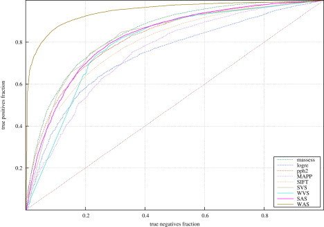
ROC Curves Produced by the Five Tools and the Four Integrated Scores with the HumVar Dataset
Figure 2.
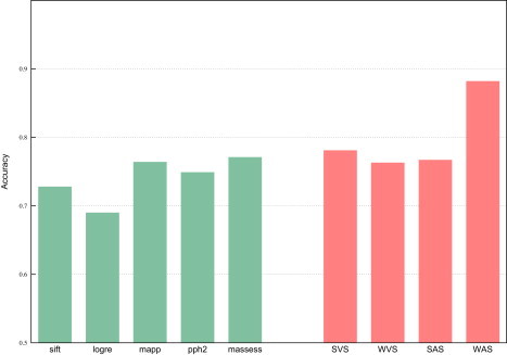
Accuracy with which the Five Tools and the Four Integrated Scores Classify the Hum Var Dataset
Green bars: accuracy of individual methods. Red bars: accuracy of integrated scores.
Both the original five tools and the four integrated scores were better at classifying HumDiv than HumVar. This behavior came as no surprise given the composition of both datasets. They contain disease-related SNVs as positive examples; however, whereas the negative examples in HumVar are common human polymorphisms, HumDiv contains observed amino acid changes in mammalian orthologous proteins. Because all the five tools (and, consequently, the integrated results) are designed to distinguish between amino acid changes that are probably deleterious and those that are accepted in evolution, the negative examples in HumDiv are as a rule awarded lower scores than their HumVar counterparts, whose alterations are not necessarily found in orthologous proteins. This is why we give higher relevance to the results obtained with HumVar (where the improvement of the WAS with respect to the individual methods is more notable) and use the weights computed from this dataset in the remaining parts of this work. For the same reason, the complementary cumulative distributions of scores distributed with the script that calculates the WAS (see last section of the Discussion) correspond to HumVar mutations.
We recalculated the WAS for all HumVar mutations by using the weights computed from the tools' classification of HumDiv. We have called this process cross-classification, and we employed it as a means of validating the WAS approach on a dataset different than the one used for computing the weights. (The complementary cross-classification was also performed.) Figure S7 presents the ROC curves resulting from cross-classification of both datasets along with the original ROC curves. It is apparent from this graph that the accuracy of HumVar cross-classification is practically equal to that of to its self-classification. On the other hand, cross-classifying HumDiv decreases the accuracy of the WAS on this dataset by only approximately 2%.
We also performed a 10-fold cross-validation of the WAS on HumVar (Figure S7). The ROC curve resulting from this cross-validation shows that very little accuracy is lost when the weights are computed from 90% of the mutations in HumVar and used for classification of the remaining 10%.
Cancer Mutation Recurrence Correlates with WAS
Because the WAS exhibited the best performance in the task of classifying the mutations in HumVar and HumDiv, we then evaluated whether the WAS could be used as an indicator of the importance of cancer-associated mutations. For that we assessed how well it correlated with cancer mutation recurrence. To perform the analysis, we sampled four disjoint subsets of Cosmic mutations with increasing recurrence: mutations appearing in only one sample, mutations recurring in two to four samples, mutations recurring in five to nine samples, and those appearing in ten or more samples (see Material and Methods). We calculated two values of WAS for each mutation by using the weights obtained from the complementary cumulative distributions of deleterious and neutral mutations in HumVar.
As presented in Figure 3, the subsets of Cosmic exhibited significantly different WAS distributions, as detected by the Wilcoxon-Mann-Whitney test. The subset of mutations found in only one sample exhibited a mean WAS of 0.538, whereas the mutations recurring in ten or more samples presented a mean WAS of 0.706. The p value corresponding to the comparison of the extreme groups was 2.33 × 10−143. In contrast, neutral polymorphisms from HumVar present a mean WAS of 0.236, and their comparison to all groups of cancer mutations produced p values smaller than 10−318.
Figure 3.
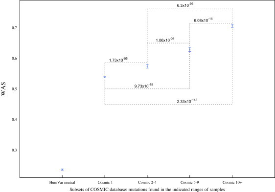
Comparison of the WAS of Four Disjoint Sets of Mutations from the Cosmic Database and the WAS of HumVar Neutral Mutations
The five sets consist, respectively, of the neutral mutations in HumVar, the mutations appearing in only one sample (1), those appearing in two to four samples (2–4), those appearing in five to nine samples (5–9), and those appearing in ten or more samples (10+) in the Cosmic database. The points represent the mean WAS; the error bars represent the standard error of the mean. The weights were computed from the HumVar dataset. The p values resulting from the Wilcoxon-Mann-Whitney test of each group-group comparison are shown in the graph. (All comparisons including neutral polymorphisms yielded p values smaller than 10−318.)
We made the same comparisons by using the WAS computed with the weights taken from HumDiv (Figure S8). We found that the mean WAS of the four groups tended to be smaller, and the differences were not so well marked as with the HumVar WAS. The better results obtained with the HumVar WAS are most likely explained by the deleterious mutations and neutral polymorphisms in HumVar—and therefore the distribution of their scores—are more similar to highly recurrent and nonrecurrent cancer mutations than the Mendelian-disease-related mutations and orthologous amino acid changes that compose HumDiv.
The WAS Correlates with the Biological Activity of TP53 Mutants
In an attempt to determine whether the WAS could serve as a good predictor of the impact of different missense mutations on the biological activity of proteins, we examined the correlation between the average WAS and the activity of the mutant protein. For this analysis we used a dataset composed of more than two thousand TP53 mutants and their associated biological activity measured as the trans-activation of transcription at four yeast promoters.
The mutants in the TP53 database were binned by their biological activity (as a percentage of the wild-type) at four yeast promoters, WAF1, MDM2, AIP1, and NOXA.31–33 We formed ten bins by grouping the mutants with activity between 0% and 10% of the wild-type, between 10% and 20%, and so on. We then evaluated to what degree the WAS of the mutations in each bin correlated with the higher activity of the bin (Figure 4). We found that the decrease in the ability of the p53 mutants to stimulate transcription with respect to the wild-type shows a high anti-correlation to the WAS of the bins. The Pearson's correlation coefficient ranged from −0.9 to −0.94.
Figure 4.
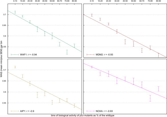
Correlation between the WAS and the Biological Activity of Bins of _TP_53 Mutants
Mutants' activity measured as their ability to trans-activate transcription at four yeast promoters (WAF1, MDM2, AIP1, and NOXA) is given as a percent of the wild-type activity. The points represent the mean WAS; the error bars represent the standard error of the mean.
A positional analysis of the WAS of mutants occurring in the DNA binding domain of p53 revealed that positions 175, 176, 179, 196, 242, 248, 278, and 282 exhibited mean values of WAS with p values below 0.005 (Figure 5). In other words, the probability that such mutations are neutral is lower than 0.5%, as deduced from the complementary cumulative distribution of HumVar neutral mutations.
Figure 5.
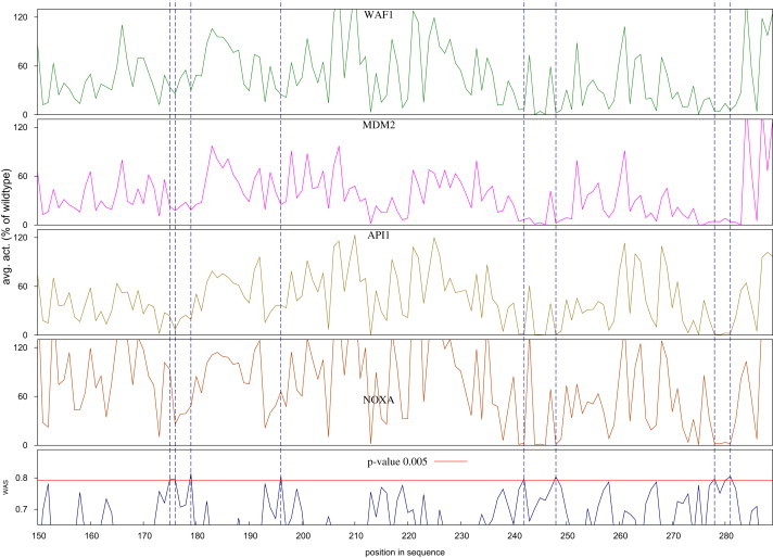
Mutational Landscape of the C-Terminal Half of the DNA-Binding Domain of p53
The abscissa of all graphs represents the position within the sequence. The bottom graph depicts the mean WAS of mutants at each position, and the other four graphs contain the mean biological activity, measured as the trans-activation of transcription at four yeast promoters (WAF1, MDM2, AIP1, and NOXA, from top to bottom). Only 0.5% of the neutral mutations in HumVar score at or above the WAS value marked by the red line in the bottom graph; vertical broken lines show the positions with mean WAS greater than this value.
Discussion
Designing and Implementing a Consensus Deleteriousness Score
In this work we integrated the output of five classifiers that categorize SNVs as probably neutral or probably deleterious. Others have employed this idea in bioinformatics to accomplish tasks such as the identification of functional elements within the genome.34–36 We devised a simple approach, consisting of classifying two very comprehensive datasets of human mutations, both neutral and deleterious, with five of the most widely employed computational tools for sorting missense SNVs.7–9,12–15,18,19,23 The basic idea behind the integration of these tools is to take advantage of their possible complementary performance at classifying missense SNVs. An example of this complementarity can be appreciated in the fact that although SIFT, PPH2, and Massessor misclassify between 24.7% and 46.4% of HumVar neutral mutations, only 13.5% are misclassified by all three (Figure S9).
We combined the outputs of SIFT, Logre, MAPP, PPH2, and Massessor by using two naive (SVS and WVS) and two weighted approaches (SAS and WAS). We found that the WAS performed better that the SAS in the task of classifying missense mutations as neutral or deleterious, as expected. On the other hand, the SVS actually outperforms its weighted counterpart by 2% in HumVar. All the gain occurs at low scores, and it is most likely caused by the different denominator used for calculating the SVS and the WVS. Whereas the SVS divides the summation by the number of tools that successfully classified the mutation, the WVS divides it by the sum of their weights. As a result, at lower scores—corresponding to mutations classified as neutral by most methods—the SVS actually receives a greater penalty than the WVS and separates the populations of deleterious and neutral mutations better.
The WAS attains an accuracy of 88.2% for classifying HumVar and 89.6% for classifying HumDiv. It outperforms all individual tools and the other three integrated scores at this task. This behavior makes it the combination of choice for integrating the output of tools aimed at classifying the outcome of missense mutations. As cited in the Results section, the higher accuracy reached by the HumDiv WAS is actually an artifact of the composition of the dataset. Therefore, we recommend that the weights calculated from HumVar be used to compute the WAS of missense SNVs, both for the task of classifying them as deleterious or neutral, and for that of ranking their deleteriousness.
We also tested the performance of the WAS at categorizing subsets of mutations classified by exactly the same number of tools to make sure that the WAS was not biased toward sets of mutations recognized by more tools. Figure S10 shows that the ROC curves produced by the WAS on the subsets of HumVar and HumDiv mutations classified by exactly five tools are very similar to those of the entire datasets. The accuracy of the WAS in the subset of HumDiv mutations classified by only four tools is slightly better than its accuracy for the whole dataset. Probably a lower fraction of mutations incoherently classified by several tools appears within this subset than in the entire dataset. (Analogous results were obtained for mutations classified by exactly four tools.)
WAS Used as a Deleteriousness Score
For the above-stated reasons, we chose the WAS computed from HumVar weights to proceed to score sets of differently recurring cancer mutations and p53 mutants (see Material and Methods). We wanted to assess whether, in addition to performing well at sorting neutral from deleterious mutations, the WAS would behave as a good predictor of the effect of different mutations on the biological activity of the mutants. In other words, we intended to test whether the WAS could be used as a deleteriousness score of mutations. The underlying hypothesis was that more-deleterious amino acid changes should coherently be awarded high scores by all methods, thus resulting in higher WAS values.
In agreement with this thought, we found that more-recurrent cancer mutations possess significantly higher WAS values than their nonrecurrent counterparts. Moreover, the average WAS increases with the number of samples in which a mutation is found. It also correlates very well with the decrease in biological activity of p53 mutants. Three of the positions with WAS p values below 5 × 10⁻³ (175, 248, and 282) correspond to known p53 mutation hotspots. Amino acid changes at the first and last position are classified as “structural” mutations, whereas the 248 position (occupied by an arginine in the wild-type protein) is a “contact” residue.32,37,38 Changes at these three positions result in mutants whose trans-activation capability is severely impaired (as shown in the upper panels of Figure 4). Interestingly, the other five positions with significantly high average WAS, although not recognized as p53 mutational hotspots, do harbor mutants, which exhibit sharp decreases of their trans-activation capacity. Taken together, these results indicate that the WAS may indeed serve as a good indicator of the decrease in biological activity resulting from a missense deleterious mutation.
Using Condel
Given the above results, we propose that research groups interested in assessing the probability that a set of missense SNVs is deleterious run the five tools used in this work and integrate their resulting scores by using a WAS-type approach. (To accomplish this first step, groups need not download and install the five tools locally. Instead, they may query each tool at its webserver; the URLs are listed in the Web Resources.) This probability-based integration, which relies on the consistency of the assessment made by different methods, should be of interest, primarily to groups embarked in genome-wide projects producing large catalogs of missense SNVs. To facilitate the employment of our integration approach, which we have named Condel, we have made available a PERL script that computes the WAS of missense mutations from the complementary cumulative distributions of scores of deleterious and neutral mutations in HumVar. This PERL script, along with the files containing such complementary cumulative distributions, is available from our group's website (see Web Resources).
Examples of projects that could benefit from the use of Condel include The Cancer Genome Atlas, the International Cancer Genome Consortium, the 1000 Genomes Project Consortium, and the sequencing of genomes of patients affected by rare diseases. In particular, projects of this latter type, which frequently require ranking de novo single-nucleotide variants found in exomic sequences by their potential effect on protein function, should find Condel very useful.
The simplicity of Condel allows it to be easily modified to include the output of new methods to the integrated score or to change the datasets from which the weights are calculated. The former requires only a modification of the PERL script provided at our website and the calculation of the complementary cumulative distributions corresponding to the new tool, and the latter needs the recalculation of the complementary cumulative distributions. It can be used with a subset of the five methods and yield very good results, as shown in Figure S10.
Acknowledgments
We would like to thank Xavier Rafael, Sophia Derdak and the useful suggestions and feedback provided by anonymous reviewers, and Jordi Deu-Pons for maintenance of condel website. We acknowledge funding from the Spanish Ministerio de Educación y Ciencia, grant number SAF2009-06954 and the Spanish National Institute of Bioinformatics (INB).
Contributor Information
Abel González-Pérez, Email: abel.gonzalez@upf.edu.
Nuria López-Bigas, Email: nuria.lopez@upf.edu.
Supplemental Data
Document S1. Ten Figures and One Table
Web Resources
The URLs for data presented herein are as follows:
- Pph2, HumVar, HumDiv: http://genetics.bwh.harvard.edu/pph2/dokuwiki/downloads; http://genetics.bwh.harvard.edu/pph2
- SIFT: http://sift.jcvi.org/
- MAPP: http://mendel.stanford.edu/sidowlab/downloads/MAPP/index.html; http://www.prophyler.org/
- Logre: http://www.cgl.ucsf.edu/Research/genentech/canpredict/
- Massessor: http://mutationassessor.org
- Online Mendelian Inheritance in Man (OMIM): http://www.ncbi.nlm.nih.gov/Omim
- Condel: http://bg.upf.edu/condel
References
- 1.Cancer Genome Atlas Research Network Comprehensive genomic characterization defines human glioblastoma genes and core pathways. Nature. 2008;455:1061–1068. doi: 10.1038/nature07385. [DOI] [PMC free article] [PubMed] [Google Scholar]
- 2.Hudson T.J., Anderson W., Artez A., Barker A.D., Bell C., Bernabe R.R., Bhan M.K., Calvo F., Eerola I., Gerhard D.S. International network of cancer genome projects. Nature. 2010;464:993–998. doi: 10.1038/nature08987. [DOI] [PMC free article] [PubMed] [Google Scholar]
- 3.Durbin R.M., Abecasis G.R., Altshuler D.L., Auton A., Brooks L.D., Gibbs R.A., Hurles M.E., McVean G.A. A map of human genome variation from population-scale sequencing. Nature. 2010;467:1061–1073. doi: 10.1038/nature09534. [DOI] [PMC free article] [PubMed] [Google Scholar]
- 4.Ng S.B., Bigham A.W., Buckingham K.J., Hannibal M.C., McMillin M.J., Gildersleeve H.I., Beck A.E., Tabor H.K., Cooper G.M., Mefford H.C. Exome sequencing identifies MLL2 mutations as a cause of Kabuki syndrome. Nat. Genet. 2010;42:790–793. doi: 10.1038/ng.646. [DOI] [PMC free article] [PubMed] [Google Scholar]
- 5.Ng S.B., Buckingham K.J., Lee C., Bigham A.W., Tabor H.K., Dent K.M., Huff C.D., Shannon P.T., Jabs E.W., Nickerson D.A. Exome sequencing identifies the cause of a Mendelian disorder. Nat. Genet. 2010;42:30–35. doi: 10.1038/ng.499. [DOI] [PMC free article] [PubMed] [Google Scholar]
- 6.Ng S.B., Nickerson D.A., Bamshad M.J., Shendure J. Massively parallel sequencing and rare disease. Hum. Mol. Genet. 2010;19:R119–R124. doi: 10.1093/hmg/ddq390. [DOI] [PMC free article] [PubMed] [Google Scholar]
- 7.Adzhubei I.A., Schmidt S., Peshkin L., Ramensky V.E., Gerasimova A., Bork P., Kondrashov A.S., Sunyaev S.R. A method and server for predicting damaging missense mutations. Nat. Methods. 2010;7:248–249. doi: 10.1038/nmeth0410-248. [DOI] [PMC free article] [PubMed] [Google Scholar]
- 8.Binkley J., Karra K., Kirby A., Hosobuchi M., Stone E.A., Sidow A. ProPhylER: A curated online resource for protein function and structure based on evolutionary constraint analyses. Genome Res. 2010;20:142–154. doi: 10.1101/gr.097121.109. [DOI] [PMC free article] [PubMed] [Google Scholar]
- 9.Clifford R.J., Edmonson M.N., Nguyen C., Buetow K.H. Large-scale analysis of non-synonymous coding region single nucleotide polymorphisms. Bioinformatics. 2004;20:1006–1014. doi: 10.1093/bioinformatics/bth029. [DOI] [PubMed] [Google Scholar]
- 10.Conde L., Vaquerizas J.M., Dopazo H., Arbiza L., Reumers J., Rousseau F., Schymkowitz J., Dopazo J. PupaSuite: finding functional single nucleotide polymorphisms for large-scale genotyping purposes. Nucleic Acids Res. 2006;34:W621–W625. doi: 10.1093/nar/gkl071. [DOI] [PMC free article] [PubMed] [Google Scholar]
- 11.Ferrer-Costa C., Orozco M., de la Cruz X. Sequence-based prediction of pathological mutations. Proteins. 2004;57:811–819. doi: 10.1002/prot.20252. [DOI] [PubMed] [Google Scholar]
- 12.Kaminker J.S., Zhang Y., Watanabe C., Zhang Z. CanPredict: A computational tool for predicting cancer-associated missense mutations. Nucleic Acids Res. 2007;35:W595–W598. doi: 10.1093/nar/gkm405. [DOI] [PMC free article] [PubMed] [Google Scholar]
- 13.Kumar P., Henikoff S., Ng P.C. Predicting the effects of coding non-synonymous variants on protein function using the SIFT algorithm. Nat. Protoc. 2009;4:1073–1081. doi: 10.1038/nprot.2009.86. [DOI] [PubMed] [Google Scholar]
- 14.Ng P.C., Henikoff S. Predicting deleterious amino acid substitutions. Genome Res. 2001;11:863–874. doi: 10.1101/gr.176601. [DOI] [PMC free article] [PubMed] [Google Scholar]
- 15.Ng P.C., Henikoff S. SIFT: Predicting amino acid changes that affect protein function. Nucleic Acids Res. 2003;31:3812–3814. doi: 10.1093/nar/gkg509. [DOI] [PMC free article] [PubMed] [Google Scholar]
- 16.Reumers J., Maurer-Stroh S., Schymkowitz J., Rousseau F. SNPeffect v2.0: A new step in investigating the molecular phenotypic effects of human non-synonymous SNPs. Bioinformatics. 2006;22:2183–2185. doi: 10.1093/bioinformatics/btl348. [DOI] [PubMed] [Google Scholar]
- 17.Reumers J., Conde L., Medina I., Maurer-Stroh S., Van Durme J., Dopazo J., Rousseau F., Schymkowitz J. Joint annotation of coding and non-coding single nucleotide polymorphisms and mutations in the SNPeffect and PupaSuite databases. Nucleic Acids Res. 2008;36:D825–D829. doi: 10.1093/nar/gkm979. [DOI] [PMC free article] [PubMed] [Google Scholar]
- 18.Reva B., Antipin Y., Sander C. Determinants of protein function revealed by combinatorial entropy optimization. Genome Biol. 2007;8:R232. doi: 10.1186/gb-2007-8-11-r232. [DOI] [PMC free article] [PubMed] [Google Scholar]
- 19.Stone E.A., Sidow A. Physicochemical constraint violation by missense substitutions mediates impairment of protein function and disease severity. Genome Res. 2005;15:978–986. doi: 10.1101/gr.3804205. [DOI] [PMC free article] [PubMed] [Google Scholar]
- 20.Ferrer-Costa C., Gelpí J.L., Zamakola L., Parraga I., de la Cruz X., Orozco M. PMUT: A web-based tool for the annotation of pathological mutations on proteins. Bioinformatics. 2005;21:3176–3178. doi: 10.1093/bioinformatics/bti486. [DOI] [PubMed] [Google Scholar]
- 21.Cooper G.M., Stone E.A., Asimenos G., NISC Comparative Sequencing Program, Green E.D., Batzoglou S., Sidow A. Distribution and intensity of constraint in mammalian genomic sequence. Genome Res. 2005;15:901–913. doi: 10.1101/gr.3577405. [DOI] [PMC free article] [PubMed] [Google Scholar]
- 22.Goode D.L., Cooper G.M., Schmutz J., Dickson M., Gonzales E., Tsai M., Karra K., Davydov E., Batzoglou S., Myers R.M. Evolutionary constraint facilitates interpretation of genetic variation in resequenced human genomes. Genome Res. 2010;20:301–310. doi: 10.1101/gr.102210.109. [DOI] [PMC free article] [PubMed] [Google Scholar]
- 23.Kaminker J.S., Zhang Y., Waugh A., Haverty P.M., Peters B., Sebisanovic D., Stinson J., Forrest W.F., Bazan J.F., Seshagiri S. Distinguishing cancer-associated missense mutations from common polymorphisms. Cancer Res. 2007;67:465–473. doi: 10.1158/0008-5472.CAN-06-1736. [DOI] [PubMed] [Google Scholar]
- 24.Forbes S.A., Tang G., Bindal N., Bamford S., Dawson E., Cole C., Kok C.Y., Jia M., Ewing R., Menzies A. COSMIC (the Catalogue of Somatic Mutations in Cancer): a resource to investigate acquired mutations in human cancer. Nucleic Acids Res. 2010;38:D652–D657. doi: 10.1093/nar/gkp995. [DOI] [PMC free article] [PubMed] [Google Scholar]
- 25.Forbes S.A., Bindal N., Bamford S., Cole C., Kok C.Y., Beare D., Jia M., Shepherd R., Leung K., Menzies A. COSMIC: mining complete cancer genomes in the Catalogue of Somatic Mutations in Cancer. Nucleic Acids Res. 2010;39:D945–D950. doi: 10.1093/nar/gkq929. [DOI] [PMC free article] [PubMed] [Google Scholar]
- 26.Kato S., Han S.Y., Liu W., Otsuka K., Shibata H., Kanamaru R., Ishioka C. Understanding the function-structure and function-mutation relationships of p53 tumor suppressor protein by high-resolution missense mutation analysis. Proc. Natl. Acad. Sci. USA. 2003;100:8424–8429. doi: 10.1073/pnas.1431692100. [DOI] [PMC free article] [PubMed] [Google Scholar]
- 27.Kawaguchi T., Kato S., Otsuka K., Watanabe G., Kumabe T., Tominaga T., Yoshimoto T., Ishioka C. The relationship among p53 oligomer formation, structure and transcriptional activity using a comprehensive missense mutation library. Oncogene. 2005;24:6976–6981. doi: 10.1038/sj.onc.1208839. [DOI] [PubMed] [Google Scholar]
- 28.Vilella A.J., Severin J., Ureta-Vidal A., Heng L., Durbin R., Birney E. EnsemblCompara GeneTrees: Complete, duplication-aware phylogenetic trees in vertebrates. Genome Res. 2009;19:327–335. doi: 10.1101/gr.073585.107. [DOI] [PMC free article] [PubMed] [Google Scholar]
- 29.Do C.B., Mahabhashyam M.S., Brudno M., Batzoglou S. ProbCons: Probabilistic consistency-based multiple sequence alignment. Genome Res. 2005;15:330–340. doi: 10.1101/gr.2821705. [DOI] [PMC free article] [PubMed] [Google Scholar]
- 30.Thompson J.D., Higgins D.G., Gibson T.J. CLUSTAL W: Improving the sensitivity of progressive multiple sequence alignment through sequence weighting, position-specific gap penalties and weight matrix choice. Nucleic Acids Res. 1994;22:4673–4680. doi: 10.1093/nar/22.22.4673. [DOI] [PMC free article] [PubMed] [Google Scholar]
- 31.Olivier M., Eeles R., Hollstein M., Khan M.A., Harris C.C., Hainaut P. The IARC TP53 database: New online mutation analysis and recommendations to users. Hum. Mutat. 2002;19:607–614. doi: 10.1002/humu.10081. [DOI] [PubMed] [Google Scholar]
- 32.Olivier M., Petitjean A., Marcel V., Pétré A., Mounawar M., Plymoth A., de Fromentel C.C., Hainaut P. Recent advances in p53 research: an interdisciplinary perspective. Cancer Gene Ther. 2009;16:1–12. doi: 10.1038/cgt.2008.69. [DOI] [PubMed] [Google Scholar]
- 33.Olivier M., Hollstein M., Hainaut P. TP53 mutations in human cancers: Origins, consequences, and clinical use. Cold Spring Harb. Perspect. Biol. 2010;2:a001008. doi: 10.1101/cshperspect.a001008. [DOI] [PMC free article] [PubMed] [Google Scholar]
- 34.Allen J.E., Salzberg S.L. JIGSAW: integration of multiple sources of evidence for gene prediction. Bioinformatics. 2005;21:3596–3603. doi: 10.1093/bioinformatics/bti609. [DOI] [PubMed] [Google Scholar]
- 35.Allen J.E., Majoros W.H., Pertea M., Salzberg S.L. JIGSAW, GeneZilla, and GlimmerHMM: Puzzling out the features of human genes in the ENCODE regions. Genome Biol. 2006;7(Suppl 1: S9):1–13. doi: 10.1186/gb-2006-7-s1-s9. [DOI] [PMC free article] [PubMed] [Google Scholar]
- 36.Coghlan A., Durbin R. Genomix: A method for combining gene-finders' predictions, which uses evolutionary conservation of sequence and intron-exon structure. Bioinformatics. 2007;23:1468–1475. doi: 10.1093/bioinformatics/btm133. [DOI] [PMC free article] [PubMed] [Google Scholar]
- 37.Brázdová M., Palecek J., Cherny D.I., Billová S., Fojta M., Pecinka P., Vojtesek B., Jovin T.M., Palecek E. Role of tumor suppressor p53 domains in selective binding to supercoiled DNA. Nucleic Acids Res. 2002;30:4966–4974. doi: 10.1093/nar/gkf616. [DOI] [PMC free article] [PubMed] [Google Scholar]
- 38.Joerger A.C., Fersht A.R. Structure-function-rescue: the diverse nature of common p53 cancer mutants. Oncogene. 2010;26:2226–2242. doi: 10.1038/sj.onc.1210291. [DOI] [PubMed] [Google Scholar]
Associated Data
This section collects any data citations, data availability statements, or supplementary materials included in this article.
Supplementary Materials
Document S1. Ten Figures and One Table