Time Series Anomaly Detection Using Deep Learning - MATLAB & Simulink (original) (raw)

Main Content

This example shows how to detect anomalies in sequence or time series data.

To detect anomalies or anomalous regions in a collection of sequences or time series data, you can use an autoencoder. An autoencoder is a type of model that is trained to replicate its input by transforming the input to a lower dimensional space (the encoding step) and reconstructing the input from the lower dimensional representation (the decoding step). Training an autoencoder does not require labeled data.

An autoencoder itself does not detect anomalies. Training an autoencoder using only representative data yields a model that can reconstruct its input data by using features learned from the representative data only. To check if an observation is anomalous using an autoencoder, input the observation into the network and measure the error between the original observation and the reconstructed observation. A large error between the original and reconstructed observations indicates that the original observation contains features unrepresentative of the data used to train the autoencoder and is anomalous. By observing the element-wise error between the original and reconstructed sequences, you can identify localized regions of anomalies.

This image shows an example sequence with anomalous regions highlighted.

This example uses the Waveform data set which contains 2000 synthetically generated waveforms of varying length with three channels.

Load Training Data

Load the Waveform data set from WaveformData.mat. The observations are numTimeSteps-by-numChannels arrays, where numtimeSteps and numChannels are the number of time steps and channels of the sequence, respectively.

View the sizes of the first few sequences.

ans=5×1 cell array {103×3 double} {136×3 double} {140×3 double} {124×3 double} {127×3 double}

View the number of channels. To train the network, each sequence must have the same number of channels.

numChannels = size(data{1},2)

Visualize the first few sequences in a plot.

figure tiledlayout(2,2) for i = 1:4 nexttile stackedplot(data{i},DisplayLabels="Channel " + (1:numChannels)); title("Observation " + i) xlabel("Time Step") end

Partition the data into training and validation partitions. Train the network using the 90% of the data and set aside 10% for validation.

numObservations = numel(data); XTrain = data(1:floor(0.9numObservations)); XValidation = data(floor(0.9numObservations)+1:end);

Prepare Data for Training

The network created in this example repeatedly downsamples the time dimension of the data by a factor of two, then upsamples the output by a factor of two the same number of times. To ensure that the network can unambiguously reconstruct the sequences to have the same length as the input, truncate the sequences to have a length of the nearest multiple of 2K, where K is the number of downsampling operations.

Downsample the input data twice.

Truncate the sequences to the nearest multiple of 2^numDownsamples. So that you can calculate the minimum sequence length for the network input layer, also create a vector containing the sequence lengths.

sequenceLengths = zeros(1,numel(XTrain));

for n = 1:numel(XTrain) X = XTrain{n}; cropping = mod(size(X,1), 2^numDownsamples); X(end-cropping+1:end,:) = []; XTrain{n} = X; sequenceLengths(n) = size(X,1); end

Truncate the validation data using the same steps.

for n = 1:numel(XValidation) X = XValidation{n}; cropping = mod(size(X,1),2^numDownsamples); X(end-cropping+1:end,:) = []; XValidation{n} = X; end

Define Network Architecture

Define the following network architecture, which reconstructs the input by downsampling and upsampling the data.

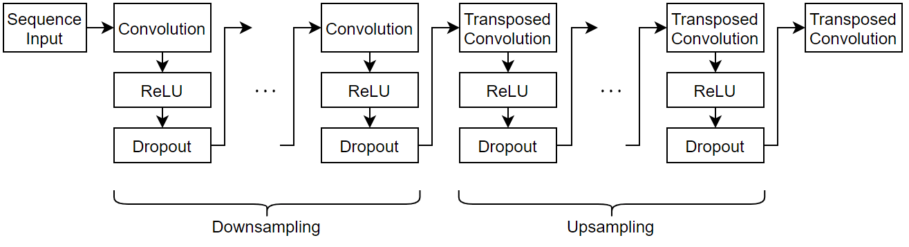
For sequence input, specify a sequence input layer with an input size matching the number of input channels. Normalize the data using Z-score normalization. To ensure that the network supports the training data, set the MinLength option to the length of the shortest sequence in the training data.
To downsample the input, specify repeating blocks of 1-D convolution, ReLU, and dropout layers. To upsample the encoded input, include the same number of blocks of 1-D transposed convolution, ReLU, and dropout layers.
For the convolution layers, specify decreasing numbers of filters with size 7. To ensure that the outputs are downsampled evenly by a factor of 2, specify a stride of 2, and set the Padding option to "same".
For the transposed convolution layers, specify increasing numbers of filters with size 7. To ensure that the outputs are upsampled evenly be a factor of 2, specify a stride of 2, and set the Cropping option to "same".
For the dropout layers, specify a dropout probability of 0.2.
To output sequences with the same number of channels as the input, specify a 1-D transposed convolution layer with a number of filters matching the number of channels of the input. To ensure output sequences are the same length as the layer input, set the Cropping option to "same".

To increase or decrease the number of downsampling and upsampling layers, adjust the value of the numDownsamples variable defined in the Prepare Data for Training section.

minLength = min(sequenceLengths); filterSize = 7; numFilters = 16; dropoutProb = 0.2;

layers = sequenceInputLayer(numChannels,Normalization="zscore",MinLength=minLength);

for i = 1:numDownsamples layers = [ layers convolution1dLayer(filterSize,(numDownsamples+1-i)*numFilters,Padding="same",Stride=2) reluLayer dropoutLayer(dropoutProb)]; end

for i = 1:numDownsamples layers = [ layers transposedConv1dLayer(filterSize,i*numFilters,Cropping="same",Stride=2) reluLayer dropoutLayer(dropoutProb)]; end

layers = [ layers transposedConv1dLayer(filterSize,numChannels,Cropping="same")];

To interactively view or edit the network, you can use Deep Network Designer.

deepNetworkDesigner(layers)

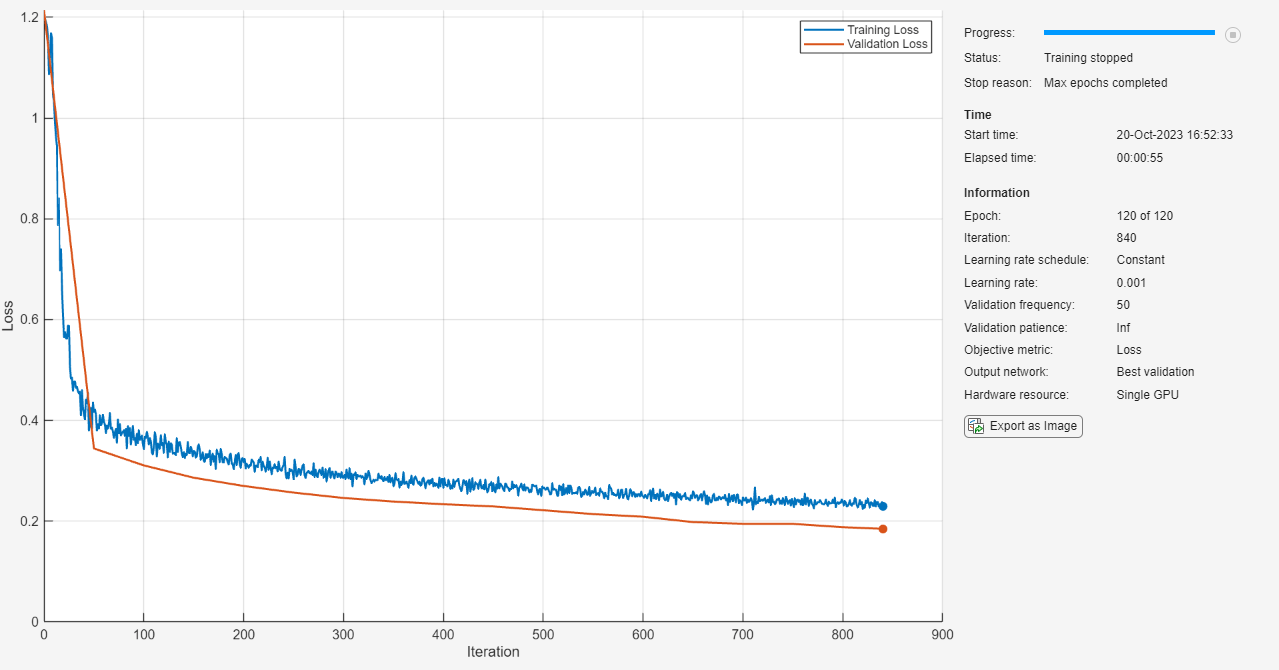
Specify Training Options

Specify the training options:

Train using the Adam solver.
Train for 120 epochs.
Shuffle the data every epoch.
Validate the network using the validation data. Specify the sequences as both the inputs and the targets.
Display the training progress in a plot.
Suppress the verbose output.

options = trainingOptions("adam", ... MaxEpochs=120, ... Shuffle="every-epoch", ... ValidationData={XValidation,XValidation}, ... Verbose=0, ... Plots="training-progress");

Train Network

Train the neural network using the trainnet function. When you train an autoencoder, the inputs and targets are the same. For regression, use mean squared error loss. By default, the trainnet function uses a GPU if one is available. Using a GPU requires a Parallel Computing Toolbox™ license and a supported GPU device. For information on supported devices, see GPU Computing Requirements (Parallel Computing Toolbox). Otherwise, the function uses the CPU. To specify the execution environment, use the ExecutionEnvironment training option.

net = trainnet(XTrain,XTrain,layers,"mse",options);

Test Network

Test the network using the validation data. Make predictions using the minibatchpredict function. By default, the minibatchpredict function uses a GPU if one is available.

YValidation = minibatchpredict(net,XValidation);

For each test sequence, calculate the root mean squared error (RMSE) between the predictions and targets. Ignore any padding values in the predicted sequences using the lengths of the target sequences for reference.

for n = 1:numel(XValidation) T = XValidation{n};

sequenceLength = size(T,1);
Y = YValidation(1:sequenceLength,:,n);

err(n) = rmse(Y,T,"all");

end

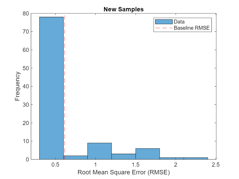
Visualize the RMSE values in a histogram.

figure histogram(err) xlabel("Root Mean Square Error (RMSE)") ylabel("Frequency") title("Representative Samples")

You can use the maximum RMSE as a baseline for anomaly detection. Determine the maximum RMSE from the validation data.

RMSEbaseline = single 0.6140

Identify Anomalous Sequences

Create a new set of data by manually editing some of the validation sequences to have anomalous regions.

Create a copy of the validation data.

Randomly select 20 of the sequences to modify.

numAnomalousSequences = 20; idx = randperm(numel(XValidation),numAnomalousSequences);

For each of the selected sequences, set a patch of the data XPatch to 4*abs(Xpatch).

for i = 1:numAnomalousSequences X = XNew{idx(i)};

idxPatch = 50:60;
XPatch = X(idxPatch,:);
X(idxPatch,:) = 4*abs(XPatch);

XNew{idx(i)} = X;

end

Make predictions on the new data.

YNew = minibatchpredict(net,XNew);

For each prediction, calculate the RMSE between the input sequence and the reconstructed sequence.

errNew = zeros(numel(XNew),1); for n = 1:numel(XNew) T = XNew{n};

sequenceLength = size(T,1);
Y = YNew(1:sequenceLength,:,n);

errNew(n) = rmse(Y,T,"all");

end

Visualize the RMSE values in a plot.

figure histogram(errNew) xlabel("Root Mean Square Error (RMSE)") ylabel("Frequency") title("New Samples") hold on xline(RMSEbaseline,"r--") legend(["Data" "Baseline RMSE"])

Identify the top 10 sequences with the largest RMSE values.

[~,idxTop] = sort(errNew,"descend"); idxTop(1:10)

ans = 10×1

Visualize the sequence with the largest RMSE value and its reconstruction in a plot.

X = XNew{idxTop(1)}; sequenceLength = size(X,1); Y = YNew(1:sequenceLength,:,idxTop(1));

figure t = tiledlayout(numChannels,1); title(t,"Sequence " + idxTop(1))

for i = 1:numChannels nexttile

plot(X(:,i))
box off
ylabel("Channel " + i)

hold on
plot(Y(:,i),"--")

end

nexttile(1) legend(["Original" "Reconstructed"])

Identify Anomalous Regions

To detect anomalous regions in a sequence, find the RMSE between the input sequence and the reconstructed sequence and highlight the regions with the error above a threshold value.

Calculate the error between the input sequence and the reconstructed sequence.

Set the time step window size to 7. Identify windows that have time steps with RMSE values of at least 10% above the maximum error value identified using the validation data.

windowSize = 7; thr = 1.1*RMSEbaseline;

idxAnomaly = false(1,size(X,1)); for t = 1:(size(X,1) - windowSize + 1) idxWindow = t:(t + windowSize - 1);

if all(RMSE(idxWindow) > thr)
    idxAnomaly(idxWindow) = true;
end

end

Display the sequence in a plot and highlight the anomalous regions.

figure t = tiledlayout(numChannels,1); title(t,"Anomaly Detection ")

for i = 1:numChannels nexttile plot(X(:,i)); ylabel("Channel " + i) box off hold on

XAnomalous = nan(1,size(X,1));
XAnomalous(idxAnomaly) = X(idxAnomaly,i);
plot(XAnomalous,"r",LineWidth=3)
hold off

end

xlabel("Time Step")

nexttile(1) legend(["Input" "Anomalous"])

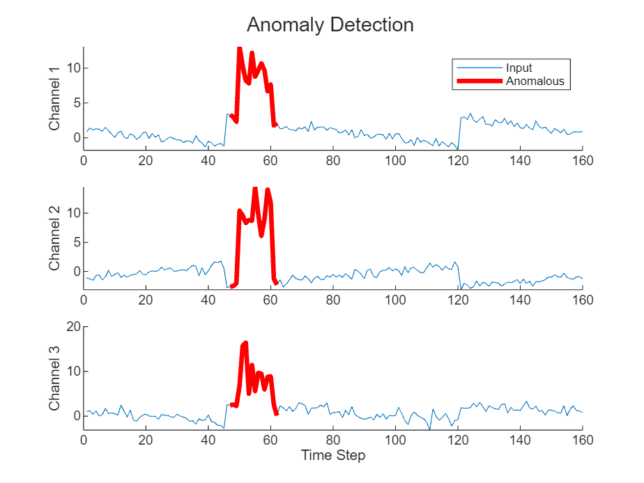
The highlighted regions indicate the windows of time steps where the error values are at least 10% higher than the maximum error value.