Image Segmentation with Mask RCNN, GrabCut, and OpenCV (original) (raw)

Last Updated : 23 Jul, 2025

Image segmentation plays a crucial role in computer vision tasks, enabling machines to understand and analyze visual content at a pixel level. It involves **dividing an image into distinct regions or objects, facilitating object recognition, tracking, and scene understanding. In this article, we explore three popular image segmentation techniques: **Mask R-CNN, **GrabCut, and **OpenCV.

Let's understand, What Image Segmentation with Mask R-CNN and GrabCut are?

What is R-CNN?

R-CNN stands for Region-based Convolutional Neural Network. It is a ground-breaking object detection system that combines object localization and recognition into an end-to-end deep learning framework.

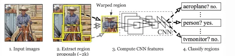
R-CNN

RNN can be summarised in the following ways.

• **Region Proposal: Initially, a region proposal algorithm (such as selective search) generates a set of potential bounding box regions in an image that are likely to contain objects of interest. These regions serve as candidate object locations.
• **Feature Extraction: Each region proposal is then individually cropped and resized to a fixed size and passed through a pre-trained CNN (such as AlexNet or VGGNet). The CNN extracts high-level features from the region, transforming it into a fixed-length feature vector.
• **Classification and Localization: The feature vector obtained from the CNN is fed into separate fully connected layers. The **classification layer predicts the probability of different object classes present in the region, while the **regression layer refines the coordinates of the bounding box, improving localization accuracy.
• **Non-Maximum Suppression (NMS): To eliminate redundant detections, non-maximum suppression is applied. It removes overlapping bounding boxes, keeping only the most confident detection for each object instance.

Mask R-CNN

Mask R-CNN (Mask Region-based Convolutional Neural Network) is a Faster R-CNN object identification framework upgrade that adds the ability to do instance segmentation. It was proposed by Kaiming He, Georgia Gkioxari, Piotr Dollár, and Ross Girshick in their work "Mask R-CNN" published in 2017.

Instance segmentation is the task of not only detecting objects in an image but also segmenting each object instance at the pixel level, providing a binary mask for each detected object. Mask R-CNN develops on Faster R-CNN's two-stage architecture with a third branch for pixel-level segmentation masks.

The following are the essential features and components of Mask R-CNN:

1. Region Proposal Network (RPN): Mask R-CNN uses an RPN to generate region proposals, just like Faster R-CNN does. The RPN generates candidate bounding boxes that are likely to contain objects of interest.
2. Region of Interest (RoI): Mask R-CNN introduces RoI Align, a more accurate technique for aligning pixel-level features within the region proposals, in place of RoI pooling used in Faster R-CNN. RoI Align ensures that the pixel-level features are accurately extracted from the original image feature map without quantization.
3. Instance Segmentation: Faster R-CNN uses two branches: classification and bounding box regression. Mask R-CNN adds a third branch that forecasts the segmentation masks for each region proposal. This branch generates a binary mask for each identified object using the RoI-aligned features as its input.

GrabCut

GrabCut is a classical algorithm of foreground extraction with minimal user interaction. It takes an input image and a user-defined bounding box that encloses the foreground object as its input (here dog is the foreground object). It then generates a refined segmentation mask that separates the foreground object from the background.

GrabCut

With an initial estimate of foreground and background regions based on the provided bounding box a Gaussian Mixture Model (GMM) is used to model the foreground and background by iteratively updating the pixel labels, improving the accuracy of the segmentation. The final output of the GrabCut algorithm is a mask image where the foreground and background regions are separated.

**Why use GrabCut and Mask R-CNN together for Image Segmentation?

Now a question arises, **Why are we using GrabCut with Mask R-CNN, isn't Mask R-CNN sufficient for image segmentation?

While Mask R-CNN is capable of producing reasonably accurate segmentation masks, there are instances where the results may contain noise or inaccuracies. This could be due to factors such as complex backgrounds, occlusions, or ambiguous object boundaries. By integrating GrabCut with Mask R-CNN, the segmentation masks can be further refined, resulting in more accurate and precise object boundaries.

Also, Combining Mask R-CNN and GrabCut can offer a more robust and accurate segmentation result. Mask R-CNN excels at automatically predicting bounding boxes and segmentation masks but may introduce subtle background artifacts. GrabCut, though requiring manual input, is effective in precise segmentation but may struggle with automation.

By using them together, you can leverage the automation of Mask R-CNN for initial segmentation and then refine it with GrabCut, benefiting from the strengths of both methods to achieve a cleaner and more accurate segmentation of foreground objects from the background. This hybrid approach balances automation and precision in image segmentation tasks.

Step-by-Step Implementation of Image Segmentation **with Mask R-CNN and GrabCut

Prerequisites

Cloning Repository for Mask RCNN

!git clone https://github.com/akTwelve/Mask_RCNN

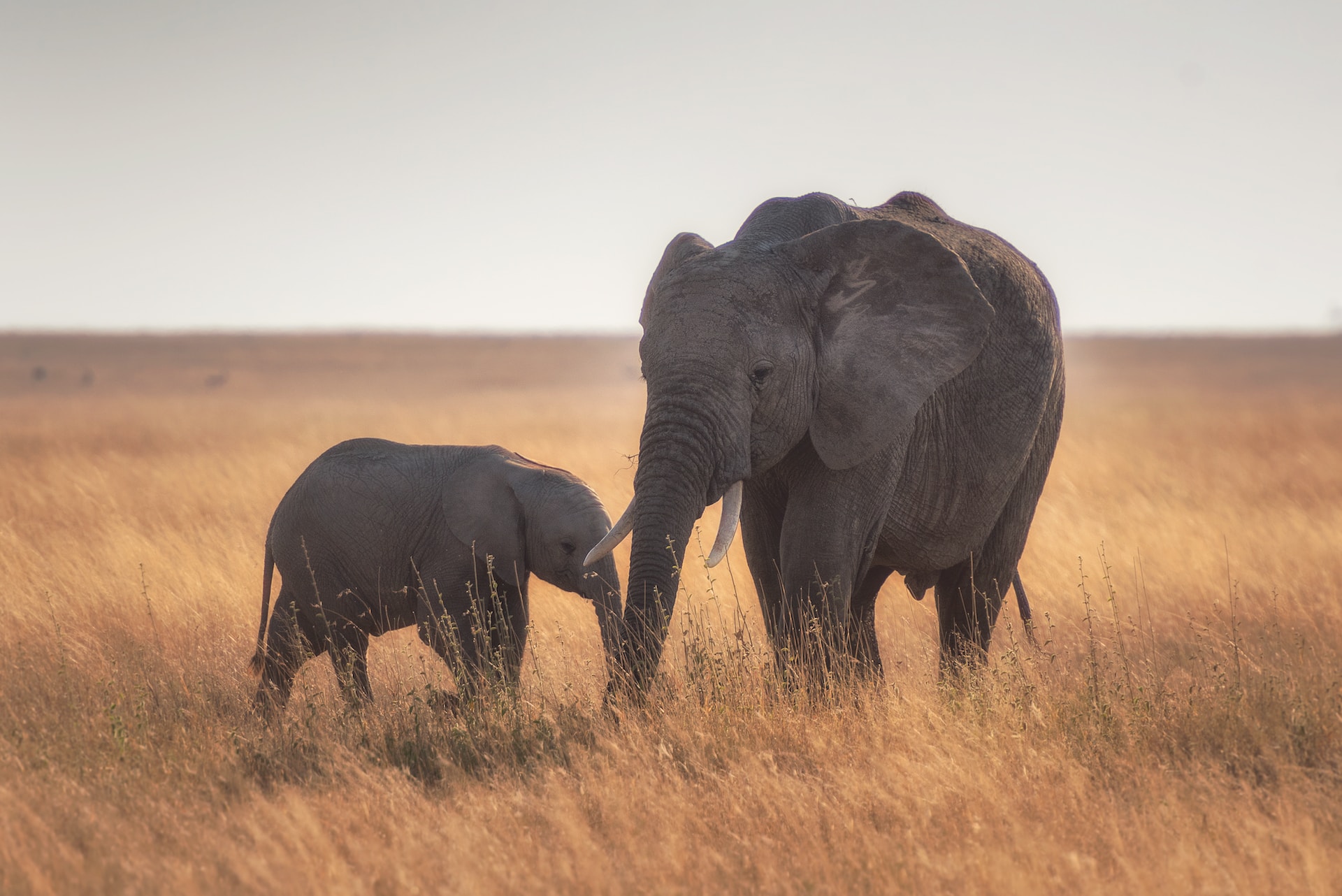
I am using this image in the implementation (Image credits: **Hu Chen)

Sample image

!wget -O image.jpg https://raw.githubusercontent.com/Anant-mishra1729/Machine-Learning-Notebooks/refs/heads/main/Mask_RCNN/image.jpg

Step 1: Importing required libraries and setting up the development environment

Python `

import os import sys import skimage.io import matplotlib.pyplot as plt import cv2 import time import numpy as np %matplotlib inline import tensorflow as tf

Root directory of the project

ROOT_DIR = "Mask_RCNN"

Import maskrcnn (mrcnn folder) as module

sys.path.append(ROOT_DIR)
from mrcnn import utils import mrcnn.model as modellib from mrcnn import visualize

Directory to save logs and trained model

MODEL_DIR = os.path.join(ROOT_DIR, "logs")

Sample image path

IMAGE_PATH = "image.jpg"

`

**Loading Model Configuration

We will use a pre-trained model, pre-trained on the MS-COCO dataset.

After downloading the pre-trained model, we will use **class InferenceConfig having parent class as **coco.CocoConfig to generate a configuration file for the model... with GPU_COUNT = 1 and IMAGES_PER_GPU = 1, we will have a BATCH SIZE = GPU_COUNT * IMAGES_PER_GPU = 1 .i.e we will provide one image at a time to GPU for inference.

Python `

For importing coco folder as module

sys.path.append(os.path.join(ROOT_DIR, "samples/coco/")) import coco

Local path to trained weights file

COCO_MODEL_PATH = os.path.join(ROOT_DIR, "mask_rcnn_coco.h5")

Download COCO trained weights from Releases if needed

if not os.path.exists(COCO_MODEL_PATH): utils.download_trained_weights(COCO_MODEL_PATH)

Loading the model configuration

class InferenceConfig(coco.CocoConfig): GPU_COUNT = 1 IMAGES_PER_GPU = 1

config = InferenceConfig() config.display()

`

**Output:

Downloading pretrained model to Mask_RCNN/mask_rcnn_coco.h5 ...
... done downloading pretrained model!
Configurations:
BACKBONE resnet101
BACKBONE_STRIDES [4, 8, 16, 32, 64]
BATCH_SIZE 1
BBOX_STD_DEV [0.1 0.1 0.2 0.2]
COMPUTE_BACKBONE_SHAPE None
DETECTION_MAX_INSTANCES 100
DETECTION_MIN_CONFIDENCE 0.7
DETECTION_NMS_THRESHOLD 0.3
FPN_CLASSIF_FC_LAYERS_SIZE 1024
GPU_COUNT 1
GRADIENT_CLIP_NORM 5.0
IMAGES_PER_GPU 1
IMAGE_CHANNEL_COUNT 3
IMAGE_MAX_DIM 1024
IMAGE_META_SIZE 93
IMAGE_MIN_DIM 800
IMAGE_MIN_SCALE 0
IMAGE_RESIZE_MODE square
IMAGE_SHAPE [1024 1024 3]
LEARNING_MOMENTUM 0.9
LEARNING_RATE 0.001
LOSS_WEIGHTS {'rpn_class_loss': 1.0, 'rpn_bbox_loss': 1.0, 'mrcnn_class_loss': 1.0, 'mrcnn_bbox_loss': 1.0, 'mrcnn_mask_loss': 1.0}
MASK_POOL_SIZE 14
MASK_SHAPE [28, 28]
MAX_GT_INSTANCES 100
MEAN_PIXEL [123.7 116.8 103.9]
MINI_MASK_SHAPE (56, 56)
NAME coco
NUM_CLASSES 81
POOL_SIZE 7
POST_NMS_ROIS_INFERENCE 1000
POST_NMS_ROIS_TRAINING 2000
PRE_NMS_LIMIT 6000
ROI_POSITIVE_RATIO 0.33
RPN_ANCHOR_RATIOS [0.5, 1, 2]
RPN_ANCHOR_SCALES (32, 64, 128, 256, 512)
RPN_ANCHOR_STRIDE 1
RPN_BBOX_STD_DEV [0.1 0.1 0.2 0.2]
RPN_NMS_THRESHOLD 0.7
RPN_TRAIN_ANCHORS_PER_IMAGE 256
STEPS_PER_EPOCH 1000
TOP_DOWN_PYRAMID_SIZE 256
TRAIN_BN False
TRAIN_ROIS_PER_IMAGE 200
USE_MINI_MASK True
USE_RPN_ROIS True
VALIDATION_STEPS 50
WEIGHT_DECAY 0.0001

**Creating a model for inference

• model = modellib.MaskRCNN(mode="inference", model_dir=MODEL_DIR, config=config)
  • The mode the parameter is set to " inference", indicating that the model will be used for inference (i.e., making predictions).
  • The model_dir parameter specifies the directory where the model weights and logs will be saved.
  • The config parameter is an instance of a configuration class (config) that determines the model's architecture and behavior.
• tf.keras.Model.load_weights(model.keras_model, COCO_MODEL_PATH, by_name=True)
  • model.keras_model accesses the underlying Keras model instance within the Mask R-CNN model.
  • **by_name=True **argument indicates that the weights should be loaded by matching layer names, allowing for partial weight loading and transfer learning. Python `

Create model object in inference mode.

model = modellib.MaskRCNN(mode="inference", model_dir=MODEL_DIR, config=config)

tf.keras.Model.load_weights(model.keras_model, COCO_MODEL_PATH, by_name=True)

`

Specifying class names

These class names will be used while visualizing the segmented objects, it performs object classification and provides class IDs as integer values to identify each class. These IDs are nothing but indices of this list.
For example: If the model detects and segments a car, then it will return **7 instead of **train, we will use this list to determine the object class as train.

Python `

class_names = ['BG', 'person', 'bicycle', 'car', 'motorcycle', 'airplane', 'bus', 'train', 'truck', 'boat', 'traffic light', 'fire hydrant', 'stop sign', 'parking meter', 'bench', 'bird', 'cat', 'dog', 'horse', 'sheep', 'cow', 'elephant', 'bear', 'zebra', 'giraffe', 'backpack', 'umbrella', 'handbag', 'tie', 'suitcase', 'frisbee', 'skis', 'snowboard', 'sports ball', 'kite', 'baseball bat', 'baseball glove', 'skateboard', 'surfboard', 'tennis racket', 'bottle', 'wine glass', 'cup', 'fork', 'knife', 'spoon', 'bowl', 'banana', 'apple', 'sandwich', 'orange', 'broccoli', 'carrot', 'hot dog', 'pizza', 'donut', 'cake', 'chair', 'couch', 'potted plant', 'bed', 'dining table', 'toilet', 'tv', 'laptop', 'mouse', 'remote', 'keyboard', 'cell phone', 'microwave', 'oven', 'toaster', 'sink', 'refrigerator', 'book', 'clock', 'vase', 'scissors', 'teddy bear', 'hair drier', 'toothbrush']

`

Inference using Mask R-CNN

Using **skimage.io.imread() we will load the image.jpg

**model.detect([image], verbose = 1) will run inference on the image and will return a dictionary with the following keys

• **rois : (ymin, xmin, ymax, xmax) coordinates of bounding box
• **masks : generated masks
• **class_ids : The resulting class ids
• **scores : Probability of class being correct.

**visualize.display_instances(image, r['rois'], r['masks'], r['class_ids'], class_names, r['scores'])

Segment Image

We will use this function to visualize the results.

Python `

#IMAGE_DIR = 'Mask_RCNN/images/'

Load a random image from the images folder

#file_names = next(os.walk(IMAGE_DIR))[2] #image = skimage.io.imread(os.path.join(IMAGE_DIR, np.random.choice(file_names))) image = skimage.io.imread("/content/image.jpg") plt.imshow(image) plt.title('Original') plt.axis('off') plt.show()

Run detection

results = model.detect([image], verbose=1)

Visualize results

r = results[0] visualize.display_instances(image, r['rois'], r['masks'], r['class_ids'], class_names, r['scores'])

`

**Output:

Processing 1 images
image shape: (1282, 1920, 3) min: 0.00000 max: 255.00000 uint8
molded_images shape: (1, 1024, 1024, 3) min: -123.70000 max: 134.10000 float64
image_metas shape: (1, 93) min: 0.00000 max: 1920.00000 float64
anchors shape: (1, 261888, 4) min: -0.35390 max: 1.29134 float32

Mask RCNN image Segmentations

Python `

For converting roi coordinates generated using Mask R-CNN

to (x1, y1, width, height)

def convertCoords(coords):

Input : (y1, x1, y2, x2)

y1, x1, y2, x2 = coords width,height = x2 - x1, y2 - y1 return (x1, y1, width, height)

Extracting masks and rois from the result

def separateEntities(r): masks = [r['masks'][:,:,i].astype("uint8") for i in range(len(r['class_ids']))] rects = [(convertCoords(roi)) for roi in r['rois']] return masks,rects

Generate masks

masks, rects = separateEntities(r)

`

Visualizing picture of masks generated using Mask R-CNN

Python3 `

Create subplots with 1 row and 2 columns

fig, (ax1, ax2) = plt.subplots(1, 2, figsize= (10,5))

Display the first mask on the left subplot

ax1.imshow(masks[0]) ax1.axis('off')

Display the second mask on the right subplot

ax2.imshow(masks[1]) ax2.axis('off')

Show the subplots

plt.show()

`

**Output:

Generated Mask

Visualizing Segmented Image using Mask R-CNN

Python3 `

Create subplots with 1 row and 2 columns

fig, (ax1, ax2) = plt.subplots(1, 2, figsize= (10,5))

Display the first mask on the left subplot

ax1.imshow(cv2.bitwise_and(image,image,mask = (r['masks'][:,:,0].astype("uint8")))) ax1.axis('off')

Display the second mask on the right subplot

ax2.imshow(cv2.bitwise_and(image,image,mask = (r['masks'][:,:,1].astype("uint8")))) ax2.axis('off')

Show the subplots

plt.show()

`

**Output:

Segmented Image

The masks generated using Mask-RCNN are not precise, there are visible background details, we will use GrabCut to remove the undesired background by refining the masks.

Applying GrabCut

GrabCut is available in OpenCV as **cv2.grabCut(img, mask, rect, bgdModel, fgdModel, iterCount, mode)

Let's explore the arguments:

1. **img: This argument represents the input image on which we want to perform the GrabCut algorithm.
2. **mask: The mask image is used to define the regions of the image as background, foreground, probable background/foreground, etc. This is achieved by assigning specific flags to different areas of the mask image. The flags used are
   1. **cv.GC_BGD (background),
   2. **cv.GC_FGD (foreground),
   3. **cv.GC_PR_BGD (probable background),
   4. **cv.GC_PR_FGD (probable foreground), or you can directly pass 0, 1, 2, or 3 to represent these regions in the image.
3. **rect: This argument represents the coordinates of a rectangle that encloses the foreground object in the format (x, y, w, h). The rectangle is used to initialize the GrabCut algorithm and provide an initial estimate of the foreground and background regions.
4. **bdgModel, fgdModel: These are numpy arrays that are internally used by the GrabCut algorithm. You need to create two zero arrays of type np.float64 and size (1, 65) to store the model parameters.
5. **iterCount: The iterCount specifies the number of iterations the GrabCut algorithm should run. More iterations can lead to better segmentation results, but at the cost of increased computation time.
6. **mode: The mode parameter determines whether we are providing the rectangle coordinates (cv.GC_INIT_WITH_RECT), mask (cv.GC_INIT_WITH_MASK), or a combination of both. This choice determines whether we are initially drawing a rectangle around the object of interest or providing additional touch-up strokes later. Python `

def applyGrabCut(image,mask,rect,iters): fgModel = np.zeros((1, 65), dtype="float") bgModel = np.zeros((1, 65), dtype="float")

apply GrabCut using the the bounding box segmentation method

(mask_grab, bgModel, fgModel) = cv2.grabCut(image, mask, rect, bgModel, fgModel, iterCount=iters, mode=cv2.GC_INIT_WITH_RECT)

values = ( ("Definite Background", cv2.GC_BGD), ("Probable Background", cv2.GC_PR_BGD), ("Definite Foreground", cv2.GC_FGD), ("Probable Foreground", cv2.GC_PR_FGD), ) valueMasks = {} for name,value in values: valueMasks[name] = (mask_grab == cv2.GC_PR_FGD).astype("uint8") * 255

return valueMasks

`

Generating Picture of Masks and Segmented image

Python `

Create subplots with 1 row and 2 columns

fig, axs = plt.subplots(2, 2, figsize=(11, 7))

Process the first mask and display the result

vm1 = applyGrabCut(image, masks[0], rects[0], 10) mother = cv2.bitwise_and(image, image, mask=vm1['Definite Foreground']) axs[0, 0].imshow(vm1['Probable Foreground']) axs[0, 0].set_title('Mother') axs[0, 0].axis('off')

Display the processed first mask

axs[0, 1].imshow(mother) axs[0, 1].set_title('Mother') axs[0, 1].axis('off')

Process the second mask and display the result

vm2 = applyGrabCut(image, masks[1], rects[1], 10) child = cv2.bitwise_and(image, image, mask=vm2['Definite Foreground']) axs[1, 0].imshow(vm2['Probable Foreground']) axs[1, 0].set_title('Child') axs[1, 0].axis('off')

Display the processed second mask

axs[1, 1].imshow(child) axs[1, 1].set_title('Child') axs[1, 1].axis('off')

Show the subplots

plt.show()

`

**Output:

Masks & Segmented image

Combining both masks

Python `

Create subplots with 1 row and 2 columns

fig, (ax1, ax2) = plt.subplots(2, 1, figsize= (8,8))

Display the combined mask

combined_mask = vm1['Definite Foreground'] | vm2['Definite Foreground'] ax1.imshow(combined_mask) ax1.axis('off') ax1.set_title('Combined Mask')

Display the second segmented image

result = mother | child ax2.imshow(result) ax2.axis('off') ax2.set_title('Segmented IMage')

Show the subplots

plt.show()

`

**Output:

You can run this implementation on Google Colab Notebook

Conclusion

In this article, we explored image segmentation using: Mask R-CNN, GrabCut, and OpenCV. Mask R-CNN utilizes deep learning to achieve pixel-level segmentation accuracy, while GrabCut offers an interactive and efficient approach. OpenCV provides a versatile library for implementing various segmentation algorithms. By understanding the strengths and limitations of each technique, developers can choose the most suitable method for their specific image segmentation needs.