Bayes Theorem in Machine learning (original) (raw)

Last Updated : 31 Dec, 2025

Bayes Theorem explains how to update the probability of a hypothesis when new evidence is observed. It combines prior knowledge with data to make better decisions under uncertainty and forms the basis of Bayesian inference in machine learning.

Handles uncertainty and noisy data effectively
Supports probabilistic interpretation of model predictions
Enables learning even with limited data
Plays a key role in real-world applications such as risk analysis and diagnosis

Mathematical Formulation of Bayes Theorem

Bayes Theorem describes the relationship between conditional probabilities and is mathematically expressed as:

P(A \mid B) = \frac{P(B \mid A) P(A)}{P(B)}

where

Posterior Probability P(A \mid B): the updated probability of hypothesis A after observing evidence B
**Likelihood P(B \mid A): the probability of observing evidence B assuming hypothesis A is true.
**Prior ProbabilityP(A): the initial belief about hypothesis A before observing any evidence.
****Evidence (Marginal Likelihood)**P(B): the total probability of observing evidence B acting as a normalization factor.

Bayes Theorem for Multiple Hypotheses (n Events)

For a set of mutually exclusive and collectively exhaustive hypotheses \{ E_1, E_2, \dots, E_n \} and an observation O the generalized Bayes’ Theorem is given by:

P(E_i \mid O) = \frac{P(O \mid E_i) P(E_i)}{\sum_{j=1}^{n} P(O \mid E_j) P(E_j)}

where

P(E_i \mid O) is the posterior probability of hypothesis E_i
P(O \mid E_i) is the likelihood of observing O under hypothesis E_i
P(E_i) is the prior probability of E_i

Step By Step Implementation

Here in this code we implements a Naive Bayes classifier that uses Bayes Theorem to compute the probability of a message being spam or ham based on word frequencies trains the model on labeled data, evaluates its performance and predicts the class of new unseen messages.

Step 1: Install and Import Required Libraries

Install essential Python libraries for data handling, ML modeling and visualization
pandas is used for data manipulation
scikit-learn provides ML algorithms and evaluation metrics
matplotlib and seaborn are used for visualization Python `

pip install pandas scikit-learn matplotlib seaborn

import pandas as pd from sklearn.model_selection import train_test_split from sklearn.feature_extraction.text import CountVectorizer from sklearn.naive_bayes import MultinomialNB from sklearn.metrics import accuracy_score, confusion_matrix, classification_report import seaborn as sns import matplotlib.pyplot as plt

Step 2: Load and Preprocess the Dataset

Load the spam dataset using pandas
Convert categorical labels into numeric values

You can download dataset from here

Python `

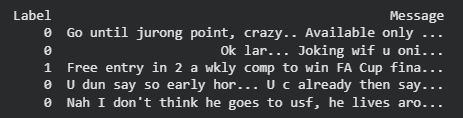
df = pd.read_csv("spam.csv", encoding='latin-1')[['v1', 'v2']] df.columns = ['Label', 'Message'] df['Label'] = df['Label'].map({'ham': 0, 'spam': 1})

print(df.head())

**Output:

bayes1

Output

Step 3: Separate Features and Target Variable

Text messages are taken as input features
Labels (0 for Ham, 1 for Spam) are the target variable Python `

X = df['Message'] y = df['Label']

Step 4: Split Data into Training and Testing Sets

Split dataset into 80% training and 20% testing
random_state ensures reproducibility Python `

X_train, X_test, y_train, y_test = train_test_split( X, y, test_size=0.2, random_state=42 )

Step 5: Convert Text Data into Numerical Form

Machine learning models cannot process raw text
CountVectorizer converts text into word frequency vectors Python `

vectorizer = CountVectorizer() X_train_vec = vectorizer.fit_transform(X_train) X_test_vec = vectorizer.transform(X_test)

Step 6: Train the Naive Bayes Model

Multinomial Naive Bayes is well-suited for text classification
Train the model using vectorized training data Python `

nb_model = MultinomialNB() nb_model.fit(X_train_vec, y_train)

Step 7: Make Predictions on Test Data

Use the trained model to predict spam or ham messages
Predictions are stored for evaluation Python `

y_pred = nb_model.predict(X_test_vec)

Step 8: Evaluate Model Performance

Calculate accuracy to measure overall performance
Generate confusion matrix for detailed analysis
Display precision, recall, and F1-score Python `

accuracy = accuracy_score(y_test, y_pred) print(f"Accuracy: {accuracy*100:.2f}%")

cm = confusion_matrix(y_test, y_pred) sns.heatmap(cm, annot=True, fmt='d', cmap='Blues', xticklabels=['Ham', 'Spam'], yticklabels=['Ham', 'Spam']) plt.title("Confusion Matrix") plt.xlabel("Predicted") plt.ylabel("Actual") plt.show()

print(classification_report(y_test, y_pred))

**Output:

Bayes2

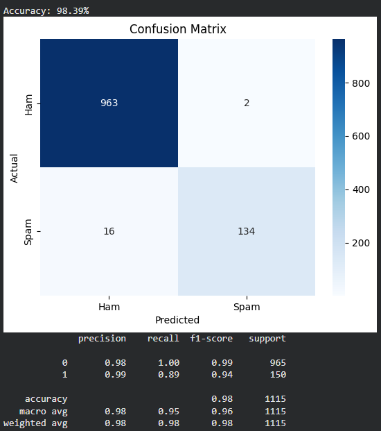
Output

Step 9: Test the Model on New Messages

Use the trained model to classify unseen messages
Vectorize new messages using the same vocabulary Python `

new_messages = [ "Congratulations! You won a free ticket.", "Hey, are we still meeting today?" ]

new_vec = vectorizer.transform(new_messages) predictions = nb_model.predict(new_vec)

for msg, pred in zip(new_messages, predictions): label = "Spam" if pred == 1 else "Ham" print(f"Message: '{msg}' => Prediction: {label}")

**Output:

Message: 'Congratulations! You won a free ticket.' => Prediction: Spam
Message: 'Hey, are we still meeting today?' => Prediction: Ham

You can download full code from here

Applications of Bayes Theorem in Machine Learning

Bayes Theorem ability to handle uncertainty and incorporate prior knowledge allows models to make accurate predictions even with incomplete or noisy data like:

**1. Naive Bayes Classifier: It is a simple probabilistic model based on Bayes’ theorem that assumes feature independence, making it efficient and effective for tasks like text classification and spam detection.

**2. Bayes optimal classifier: The Bayes optimal classifier is a theoretical model that predicts the class with the highest posterior probability for given features, representing the best possible classification accuracy. It uses Bayes’ theorem to update probabilities based on new evidence.

\hat{y} = \arg \max_{y} P(y \mid x)

where

\hat{y}: Predicted class label
y: Possible class label
x: Input feature vector
P(y \mid x)Posterior probability of class given features

**3. Bayesian Optimization: Bayesian Optimization is a technique for efficiently finding the maximum or minimum of expensive to evaluate functions using a probabilistic model often a Gaussian process. It iteratively selects the most promising points to evaluate, making it ideal for tasks like hyperparameter tuning in machine learning.

**4. Bayesian Belief Networks (BBNs): Bayesian Belief Networks (BBNs) or Bayesian networks are probabilistic graphical models that represent variables and their conditional dependencies using a directed acyclic graph (DAG). They are widely applied in risk analysis, diagnostics and decision-making.