Create a Correlation Matrix using Python (original) (raw)
Last Updated : 28 Jul, 2025
**Correlation matrix is a table that shows how different variables are related to each other. Each cell in the table displays a number i.e. correlation coefficient which tells us how strongly two variables are together. It helps in quickly spotting patterns, understand relationships and making better decisions based on data.
**A correlation matrix can be created using two libraries:
**1. Using NumPy Library
NumPy provides a simple way to create a correlation matrix. We can use the **np.corrcoef() function to find the correlation between two or more variables.
**Example: A daily sales and temperature record is kept by an ice cream store. To find the relationship between sales and temperature, we can utilize the NumPy library where x is sales in dollars and y is the daily temperature.
Python `
import numpy as np x = [215, 325, 185, 332, 406, 522, 412, 614, 544, 421, 445, 408], y = [14.2, 16.4, 11.9, 15.2, 18.5, 22.1, 19.4, 25.1, 23.4, 18.1, 22.6, 17.2] matrix = np.corrcoef(x, y) print(matrix)
`
**Output:
[[1. 0.95750662]
[0.95750662 1. ]]
**2. Using Pandas library
Pandas is used to create a correlation matrix using its built-in **corr() method. It helps in analyzing and interpreting relationships between different variables in a dataset.
**Example: Let's create a simple DataFrame with three variables and calculate correlation matrix.
Python `
import pandas as pd data = { 'x': [45, 37, 42, 35, 39], 'y': [38, 31, 26, 28, 33], 'z': [10, 15, 17, 21, 12] } dataframe = pd.DataFrame(data, columns=['x', 'y', 'z']) print("Dataframe is : ") print(dataframe) matrix = dataframe.corr() print("Correlation matrix is : ") print(matrix)
`
**Output:
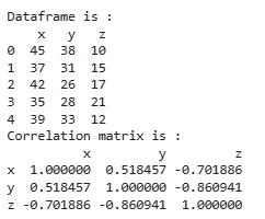
Using Pandas
3. Using Matplotlib and Seaborn for Visualization
In addition to creating a correlation matrix, it is useful to visualize it. Using libraries like Matplotlib and Seaborn, we can generate heatmaps that provide a clear visual representation of how strongly variables are correlated.
Python `
import seaborn as sns import matplotlib.pyplot as plt
matrix = dataframe.corr()
plt.figure(figsize=(8,6)) sns.heatmap(matrix, annot=True, cmap="coolwarm", fmt=".2f", linewidths=0.5) plt.title("Correlation Heatmap") plt.show()
`
**Output:
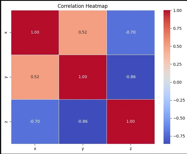
Heatmap
**Example with Real Dataset (Iris Dataset)
In this example we will consider **Iris dataset and find correlation between the features of the dataset.
- **dataset = datasets.load_iris(): Loads the Iris dataset, which includes flower feature data and species labels.
- **dataframe["target"] = dataset.target: Adds a target column to the DataFrame containing the species labels.
- **dataframe.corr(): Computes the correlation matrix for the numerical features in the DataFrame.
- **plt.figure(figsize=(8,6)): Sets the figure size to 8 inches by 6 inches.
- **sns.heatmap(matrix, annot=True, cmap="coolwarm", fmt=".2f", linewidths=0.5): Plots the correlation matrix as a heatmap, displaying values with two decimal places, using a color scale from blue (negative correlation) to red (positive correlation) and adds lines between cells for clarity. Python `
from sklearn import datasets import pandas as pd import seaborn as sns import matplotlib.pyplot as plt
dataset = datasets.load_iris() dataframe = pd.DataFrame(data=dataset.data, columns=dataset.feature_names) dataframe["target"] = dataset.target
matrix = dataframe.corr()
plt.figure(figsize=(8,6)) sns.heatmap(matrix, annot=True, cmap="coolwarm", fmt=".2f", linewidths=0.5) plt.title("Iris Dataset Correlation Heatmap") plt.show()
`
**Output:

Using IRIS dataset
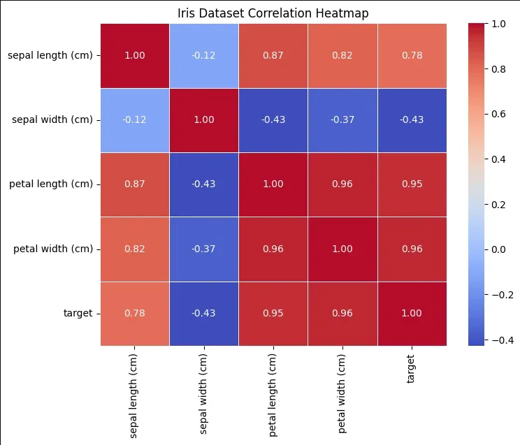
Heatmap
Understanding Correlation Values
- **No Correlation: A correlation value of 0 means no linear relationship between the variables. As one changes, the other does not follow any predictable pattern.
- **Positive Correlation: A value closer to +1 indicates a direct relationship as one variable increases, the other also increases. Example: height and weight.
- **Negative Correlation: A value closer to -1 indicates an inverse relationship as one variable increases, the other decreases. Example: speed and travel time.