LMNs Linear Algebra (original) (raw)
Last Updated : 23 Jul, 2025
Linear algebra is the study of linear combinations. It is the study of vector spaces, lines and planes, and some mappings that are required to perform the linear transformations. It includes vectors, matrices and linear functions.
Table of Content
- Vector Space
- Subspaces
- Basis and Dimension in Vector Space
- Linear Independence and dependence of vectors
- Matrices
- Determinant and Inverse of Matrices
- Null Space and Nullity
- Types of Matrices
- System of Linear Equations
- Gaussian Elimination
- Eigenvalues and Eigenvectors
- LU Decomposition
- Singular Value Decomposition
**Vector Space
- A vector space (or linear space) is a set of vectors along with two operations: vector addition and scalar multiplication.
- These operations must satisfy specific axioms, and the scalars are usually real numbers, but can also be rational, complex, etc.
**Key Operations in a Vector Space:
- Vector Addition: Takes two vectors u and v from the vector space V, and produces a third vector u+v∈V.
- Scalar Multiplication: Takes a scalar c∈F and a vector u∈V, producing a new vector cu∈V.
**Axioms of Vector Space: A vector space V must satisfy the following 10 axioms for any vectors x,y,z ∈V and scalars a,b ∈F :
- Closed Under Addition: x+y ∈V .
- Closed Under Scalar Multiplication: ax ∈V .
- Commutativity of Addition: x+y = y+x.
- Associativity of Addition: (x+y)+z = x+(y+z).
- Existence of the Additive Identity: There exists 0∈V such that x+0 = x.
- Existence of the Additive Inverse: For every x∈V, there exists −x∈V such that x+(−x) = 0.
- Existence of the Multiplicative Identity: There exists 1∈F1 such that 1⋅x = x.
- Associativity of Scalar Multiplication: a(bx) = (ab)x.
- Distributivity of Scalar Multiplication over Vector Addition: a(x+y) = ax+ay.
- Distributivity of Scalar Multiplication over Scalar Addition: (a+b)x = ax+bx.
**Examples of Vector Spaces:
- Real Numbers (ℝ): The set of all real numbers is a vector space under regular addition and scalar multiplication.
- Euclidean Space (ℝⁿ): The set of all n-tuples of real numbers (e.g.,\mathbb{R}^3 for 3-dimensional space).
- Matrices
Subspaces
A subspace W of a vector space V is a subset of V that is itself a vector space, satisfying:
- Contains the zero vector.
- Closed under addition.
- Closed under scalar multiplication.
Example:
In \mathbb{R}^2, the set of all vectors of the form (x,0) (i.e., all vectors along the x-axis) is a subspace
Basis and Dimension in Vector Space
**Basis of Vector Space:
A collection of vectors B = \{v_1, v_2, ..., v_r\} is a basis for a vector space V if it is linearly independent and spans V, meaning every vector in V can be expressed as a linear combination of the vectors in B.
Example : Standard Basis in R^2 :
e_1=(1,0) e_2=(0,1)
this are the basis of R^2
**Dimension of a Vector Space:
Number of vectors in a basis for V is called the dimension of V.
**Example: 1) dim (R^3) = 3.
- dim of matrix of order “2 × 2” is 4.
read more about Basis and Dimension of Vector Space.
Linear Independence and dependence of vectors
**Linear Independence: if a set of vectors \{v_1, v_2, ..., v_n\} is linearly independent, the only solution to the equation
c_1 v_1 + c_2 v_2 + ... + c_n v_n = 0
is when all the scalars c_1, c_2, ..., c_n are equal to zero.
**Linear Dependence: If there exists a non-trivial solution (i.e., some c_i are not zero), then the vectors are linearly dependent
**Example:
Consider the vectors v_1 = (1, 0) and v_2 = (0, 1) in \mathbb{R}^2. These vectors are linearly independent because no scalar multiple of one can produce the other.
However, for v_1 = (1, 0) and v_2 = (2, 0), they are linearly dependent because v_2 is just 2×v_1
Matrices
A matrix is a collection of numbers arranged in rows and columns. It's typically enclosed in brackets, and the size or order is denoted as "rows × columns".
**Transpose of a Matrix: The transpose of a matrix M, denoted M^T, is obtained by swapping its rows and columns. If A = [a_{ij}], then A^T = [b_{ij}] where b_{ij} = a_{ji}.
**Rank of a Matrix: The rank of a matrix is the maximum number of linearly independent rows or columns. It determines the dimension of the row space or column space.
**Example: Consider the matrix:
A = \begin{bmatrix} 1 & 2 \\ 3 & 4 \end{bmatrix} →\begin{bmatrix} 1 & 2 \\ 0 & -2 \end{bmatrix}
The matrix has 2 non-zero rows, so the rank of A is 2.
**Properties of Matrices:
- \text{tr}(A + B) = \text{tr}(A) + \text{tr}(B)
- \text{tr}(AB) = \text{tr}(BA)
- Rank properties like P(A) \leq \min(m, n)
**Trace of a Matrix: The trace is the sum of the diagonal elements of a square matrix, \text{tr}(A) = a_{11} + a_{22} + ... + a_{nn}.
Example: Consider the matrix
A = \begin{bmatrix} 3 & 4 \\ 2 & 5 \end{bmatrix}\\Tr(A)=3+5=8
Thus, the trace of matrix A is 8.
**Adjoint of a square Matrix: The adjoint of a square matrix A is the transpose of its cofactor matrix.
\text{Adj}(A) has properties like A(\text{Adj}(A)) = (\text{Adj}(A))A = |A| I.
Determinant and Inverse of Matrices
Determinant of Matrices: The determinant of a matrix represents the scaling factor of the linear transformation associated with that matrix. For example, in a 2×2 matrix, the determinant indicates how the area is scaled when the matrix transforms a shape.
Properties of Determinant:
- Transpose: \text{det}(A^T) = \text{det}(A)
- Multiplication: \text{det}(AB) = \text{det}(A) \times \text{det}(B)
- Scalar Multiplication: \text{det}(kA) = k^n \times \text{det}(A)
- Singular Matrix: {det}(A) = 0 implies A is singular.
- Adjoint Property: \text{det}(\text{adj}(A)) = \text{det}(A)^{n-1}
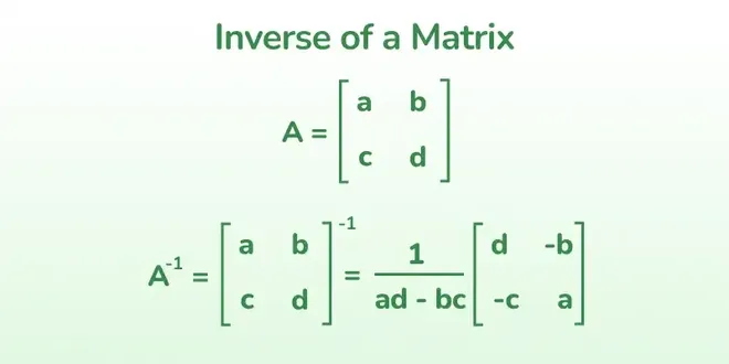
**Inverse of a Matrix: A^{-1} = \frac{\text{Adj}(A)}{|A|} (only for non-singular matrices).
Null Space and Nullity
**Null Space:
The null space of a matrix A consists of all vectors B such that A⋅B=0 , where B is not the zero vector. It represents the set of solutions to the homogeneous system of linear equations A⋅B=0, and is a subspace of the vector space.
**Nullity:
The nullity of a matrix is the dimension of its null space, representing the number of linearly independent vectors that form the null space. It indicates how many free variables exist in the solution to A⋅B=0.
**Rank-Nullity Theorem: nullity of a matrix A
Nullity of A + Rank of A = Number of columns of A
Types of Matrices
- Diagonal Matrix: All non-diagonal elements are zero.
- Identity Matrix: Diagonal elements are 1 and others are 0.
- Singular Matrix: A square matrix with a determinant of zero.
- Non-Singular Matrix: A square matrix with a non-zero determinant.
- Symmetric Matrix: A = A^T
- Skew-Symmetric Matrix: A = -A^T.
- Nilpotent Matrix: A square matrix M is called nilpotent if there exists a positive integer k such that: M^k = 0
**Orthogonal Matrix:
A square matrix A is orthogonal if its transpose is equal to its inverse, i.e., A^T = A^{-1}.
This implies:
A⋅A^T=A ^T⋅A=I
where I is the identity matrix
Properties:
- Non-Singularity: {det}(A) = ±1
- Orthogonal Diagonal Matrix: Diagonal elements are ±1
- Eigenvalues: ±1
- Eigenvectors: Eigenvectors are orthogonal to each other.
Idempotent Matrix:
An idempotent matrix is a square matrix that, when multiplied by itself, gives back the same matrix. A matrix P is said to be idempotent if P^2 = P.
Example:
The matrix given below is an idempotent matrix of order “2 × 2.”
P = \begin{bmatrix}3 & -3 \\2 & -2\end{bmatrix}
Properties:
- Square Matrix: always square matrices.
- Singular: They are singular( except identity matrix).
- Determinant: The determinant is either 0 or 1.
- Eigenvalues: The eigenvalues are either 0 or 1.
- Trace: The trace equals the rank of the matrix.
**Partition Matrix:
A Partition Matrix refers to dividing a matrix into smaller, non-overlapping submatrices (blocks)
Given the matrix:
A = \begin{bmatrix} 1 & 2 & 3 & 4 \\ 5 & 6 & 7 & 8 \\ 9 & 10 & 11 & 12 \\ 13 & 14 & 15 & 16 \end{bmatrix}
We can partition it into 4 smaller 2x2 submatrices:
\begin{bmatrix} A_{11}& A_{12} \\ A_{21} & A_{22} \end{bmatrix}
where:
A_{11} = \begin{bmatrix} 1 & 2 \\ 5 & 6 \end{bmatrix}, \quad A_{12} = \begin{bmatrix} 3 & 4 \\ 7 & 8 \end{bmatrix}A_{21} = \begin{bmatrix} 9 & 10 \\ 13 & 14 \end{bmatrix}, \quad A_{22} = \begin{bmatrix} 11 & 12 \\ 15 & 16 \end{bmatrix}
**Projection Matrix:
A matrix P is a projection matrix if
- Idempotent Property: P^2 = P .
- Square Matrix: P is a square matrix
Note: not all idempotent matrices are projection matrices. Projection matrices are a specific type of idempotent matrix, typically used to map vectors onto a subspace
System of Linear Equations
A system of linear equations is a set of equations with common variables, represented as:
\begin{aligned} a_{11}x_1 + a_{12}x_2 + \dots + a_{1n}x_n &= b_1 \\ a_{21}x_1 + a_{22}x_2 + \dots + a_{2n}x_n &= b_2 \\ &\vdots \\ a_{m1}x_1 + a_{m2}x_2 + \dots + a_{mn}x_n &= b_m \end{aligned}
The solution is the set of values (x_1, x_2, \dots, x_n) that satisfy all equations simultaneously, representing points of intersection among the equations.
**Types of Solutions:
- No Solution: The system is inconsistent, meaning no values satisfy all equations.
- Unique Solution: The system has exactly one solution.
- Infinite Solutions: The system is consistent, and the equations represent planes or lines that overlap, leading to an infinite number of solutions.
**Homogeneous Linear Equations:
AX=0 always has the trivial solution X=0.
- If the rank of A equals the number of unknowns, there is a unique solution.
- If the rank is less than the number of unknowns, there are infinite solutions.
**Non-Homogeneous Linear Equations:
AX=Bcan have different solutions based on the rank of the augmented matrix:
- If P[A:B]≠P(A)P[A:B] , there is no solution.
- If P[A:B]=P(A)= number of unknowns, there is a unique solution.
- If P[A:B]=P(A)≠ number of unknowns, there are infinite solutions.
**Consistent vs Inconsistent:
- Consistent System: A system with one or more solutions.
- Inconsistent System: A system with no solutions.
Gaussian Elimination
Gaussian elimination is a method for solving a system of linear equations by transforming the system's matrix into an upper triangular matrix and then performing back substitution to find the solution.
Steps:
- Write the system of equations in augmented matrix.
- Apply row operations
- Reduce to Row Echelon Form: The leading coefficient in each row should be 1, and zeros should be below it.
- Back substitution: Solve for each variable starting from the last equation.
**Example: Solve the system: x+y=5x , 2x−y=1
augmented matrix:\begin{bmatrix} 1 & 1 & | & 5 \\ 2 & -1 & | & 1 \end{bmatrix}
Eliminate x from second row:Perform R_2→R_2−2R_1
\begin{bmatrix} 1 & 1 & | & 5 \\ 0 & -3 & | & -9 \end{bmatrix}
Solve for y: y=3
Substitute y=3 into first equation to solve for x: x=2
Solution: x=2, y=3
Eigenvalues and Eigenvectors
- Eigenvector: A vector v that, when multiplied by a square matrix A, results in a scalar multiple of itself. The equation is: A v = \lambda v where \lambda is the eigenvalue.
- Eigenvalue: A scalar λ\lambdaλ that indicates how much the eigenvector is stretched or shrunk during the linear transformation.
-660.webp)
**Steps to Find Eigenvalues and Eigenvectors
**Find Eigenvalues:
Solve the characteristic equation \text{det}(A - \lambda I) = 0 , where I is the identity matrix and \lambda represents the eigenvalue.
**Find Eigenvectors:
For each eigenvalue \lambda, solve (A - \lambda I) v = 0 to find the corresponding eigenvector v.
Properties of Eigenvalues:
- Eigenvalues of real symmetric and Hermitian matrices are real.
- Eigenvalues of real skew-symmetric and skew-Hermitian matrices are either pure imaginary or zero.
- Eigenvalues of unitary and orthogonal matrices are of unit modulus, i.e., ∣λ∣=1.
- For a scalar multiple of a matrix kA, the eigenvalues are scaled by k: k\lambda_1, k\lambda_2, \dots
- Eigenvalues of A^{-1} are the reciprocals of the eigenvalues of A: \frac{1}{\lambda_1}, \frac{1}{\lambda_2}, \dots
- Eigenvalues of A^k are the eigenvalues raised to the power k: \lambda_1^k, \lambda_2^k, \dots
- Eigenvalues of A are the same as those of A^T (transpose).
- Sum of eigenvalues = Trace of A .
- Product of eigenvalues = determinant of A.
read more about Eigenvalues and Eigenvectors.
**LU Decomposition
LU Decomposition (or LU Factorization) is the process of decomposing a square matrix A into the product of two matrices:
A=L⋅U
where L is a lower triangular matrix (with ones on the diagonal) and U is an upper triangular matrix.
Steps:
- Matrix Setup: Convert into matrix form AX=C
- Gauss Elimination: Use Gaussian elimination to reduce matrix A to an upper triangular matrix U.
- Find L:
- Solve the System: Once you have L and U, solve the system by first solving LZ=C for Z, and then solving UX=Z for X.
Singular Value Decomposition
Singular Value Decomposition (SVD) is a method of factorizing a matrix A into three matrices:
A=UΣV^T
where:
- U is an orthogonal matrix (left singular vectors).
- Σ is a diagonal matrix containing the singular values.
- V^T is the transpose of an orthogonal matrix (right singular vectors).
Steps to Compute SVD:
- Compute AA^T
- Find Eigenvalues
- Find Right Singular Vectors
- Compute Left Singular Vectors: Use the formula u_i = \frac{1}{\sigma_i} A v_i to find the left singular vectors U.
- Construct SVD: After finding U, Σ, and V, write the decomposition A=UΣV^T.