Probability Distributions in Data Science (original) (raw)
Last Updated : 11 Mar, 2026
Understanding how data behaves is one of the first steps in data science. Before we dive into building models or running analysis, we need to understand how the values in our dataset are spread out and that’s where probability distributions come in.
**Example:
If you roll a fair die, the chance of getting a 6 is 1 out of 6, or 16.67%. This is a basic example of a probability distribution a way to describe the likelihood of different outcomes.
Probability Data Distributions
When dealing with complex data like customer purchases, stock prices, or weather, probability distributions help answer:
- What is most likely to happen?
- What are rare or unusual outcomes?
- Are values close together or spread out?
This helps us make better predictions and understand uncertainty.
Why Are Probability Distributions Important?
- Explain how data behaves (clustered or spread)
- Form the basis of machine learning models
- Used in statistical tests (e.g., p-value)
- Help identify outliers and make predictions
Before this, we need to understand random variables, which assign numbers to outcomes of random events (e.g., rolling a die).
Key Components of Probability Distributions
Now that we understand **random variables let's explore how we describe their probabilities using three key concepts:
**1. Probability Mass Function (PMF): Used for discrete variables (e.g., number of products bought). It gives the probability of each exact value. For example, 25% of customers buy exactly 3 products.
**2. **Probability Density Function (PDF): Used for continuous variables (e.g., amount spent). It shows how probabilities spread over a range but not the chance of one exact value since values can be infinite.
**3. **Cumulative Distribution Function (CDF): Used for both types, it shows the probability that a value is less than or equal to a certain number. For example, CDF(3) = 0.75 means 75% buy 3 or fewer products; CDF($50) = 0.80 means 80% spend $50 or less. To find the CDF we can use the formula given below:
\text{CDF: } F_X(x) = P(X \leq x) = \int_{-\infty}^x f(t) \, dt
Where F(x) is the CDF and f(t)is the PDF.
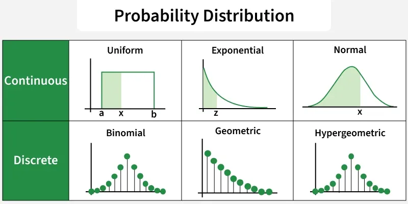
Types of Probability Distributions
Probability distributions can be divided into two main types based on the nature of the random variables: **discrete and **continuous.
**Discrete Data Distributions
A discrete distribution is used when the random variable can take on countable, specific values. For example, when predicting the number of products a customer buys in a single order the possible outcomes are whole numbers like 0, 1, 2, 3, etc. You can't buy 2.5 products so this is a discrete random variable. It includes various distributions Let's understand them one by one:
1. Binomial Distribution
The binomial distribution calculates the chance of getting a certain number of successes in a fixed number of trials.
**Formula (PMF):
P(X = k) = \binom{n}{k} p^k (1-p)^{n-k}
Where:
- n = number of trials
- k = number of successes
- p = probability of success
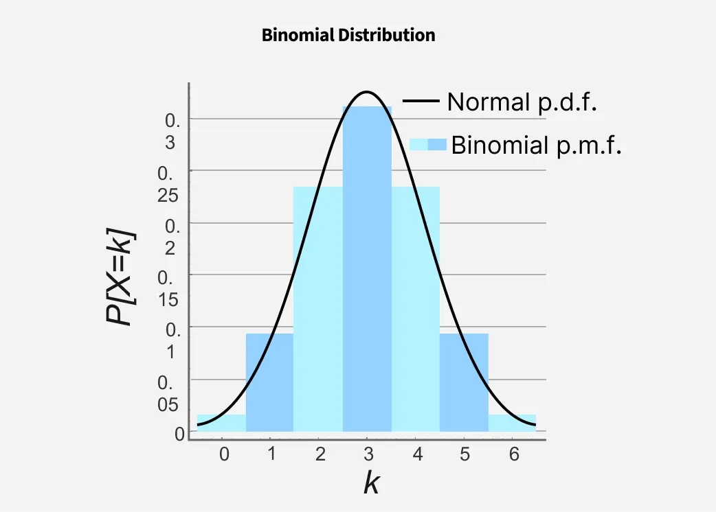
Binomial Distribution
**Example: flipping a coin 10 times and counting heads.
- Number of trials: 10
- Two outcomes per trial: heads (success) or tails (failure)
- Probability of success (heads): 0.5
- Shows likelihood of getting 0 to 10 heads
2. **Bernoulli Distribution
The Bernoulli distribution describes experiments with only one trial and two possible outcomes: success or failure. It’s the simplest probability distribution.
**Formula (PMF):
P(X = x) = p^x (1-p)^{1-x}, \quad x \in \{0,1\}

Bernoulli Distributions
**Example: flipping a coin once and checking if it lands on heads.
- One trial only
- Two outcomes: heads (success) or tails (failure)
- Probability of success: 0.5
- Graph shows two bars representing success (1) and failure (0) with equal probabilities
3. **Poisson Distribution
The Poisson distribution models the number of random events happening in a fixed time or area.
**Formula (PMF):
P(X = k) = \frac{\lambda^k e^{-\lambda}}{k!}
Where:
- λ = average rate of occurrence

Poisson Distributions
**Example:
Counting how many customers enter a coffee shop per hour. It helps predict the probability of seeing a specific number of events based on the average rate.
- Counts events in a fixed interval
- Average rate (e.g., 5 customers/hour) is known
- Calculates probability of exact counts (e.g., exactly 3 customers)
- Graph shows a curve centered around the average rate, tapering off for less likely counts
4. Geometric Distributions
The geometric distribution models the number of trials needed to get the first success in repeated independent attempts.
**Formula (PMF):
P(X = k) = (1-p)^{k-1} p

Geometric Distribution
**Example
how many emails you must send before a customer makes a purchase. It helps predict the chance of success happening at each trial.
- Counts trials until first success
- Each trial is independent with fixed success probability
- Useful for questions like “How many emails until first purchase?”
- Graph shows a decreasing curve fewer trials are more likely
Continuous Data Distributions
A **continuous distributionis used when the random variable can take any value within a specified range like when we analyze how much money a customer spends in a store then the amount can be any real number including decimals like 25.75,25.75, 25.75,50.23, etc.
In continuous distributions the **Probability Density Function (PDF) shows how the probabilities are spread across the possible values. The area under the curve of this PDF represents the probability of the random variable falling within a certain range. Now let's look at some types of continuous probability distributions that are commonly used in data science:
1. **Normal Distribution
The normal distribution, or bell curve, is one of the most common data distributions. Most values cluster around the mean, with fewer values farther away, forming a symmetrical shape. It’s perfect for modeling things like people’s heights.
- Mean is the center of the curve
- Symmetrical distribution (left and right sides mirror each other)
- Standard deviation shows how spread out the data is
- Smaller standard deviation means data is closer to the mean
**PDF Formula:
f(x) = \frac{1}{\sigma \sqrt{2\pi}} \exp\left(-\frac{(x-\mu)^2}{2\sigma^2}\right)
Where:
- μ = mean
- σ = standard deviation

Normal Distribution
2. **Exponential Distribution
The exponential distribution models the time between events happening independently and continuously. For example, the time between customer arrivals at a store. It helps predict how long you might wait for the next event.
- Models waiting time between events
- Average time (e.g., 10 minutes between customers) defines the rate (λ)
- Events occur independently and continuously
- Useful for predicting time until next event
**PDF Formula:
f(x) = \lambda e^{-\lambda x}, \quad x \ge 0

Exponential Distributions
While the exponential distribution focuses on waiting times sometimes we just need to model situations where every outcome is equally likely. In that case we use the **uniform distribution.
3. **Uniform Distribution
The uniform distribution means every outcome in a range is equally likely. For example, rolling a fair six-sided die or picking a random number between 0 and 1. It applies to both discrete and continuous cases.
- All outcomes have equal probability
- Discrete example: rolling a die (1 to 6)
- Continuous example: random number between 0 and 1
**PDF Formula:
f(x) = \frac{1}{b-a}, \quad a \le x \le b

Uniform Distribution
4. **Beta Distribution
In real-world problems, probabilities often change as we learn more. The Beta distribution helps model this uncertainty and update beliefs with new data. For example, it can estimate the chance a customer clicks an ad.
- Models changing probabilities between 0 and 1
- Parameters (α and β) control confidence and shape
- Commonly used in Bayesian stats and A/B testing
**PDF Formula:
f(x) = \frac{x^{\alpha-1}(1-x)^{\beta-1}}{B(\alpha,\beta)}
Where:
- α, β control the shape
- B (α, β) is the Beta function
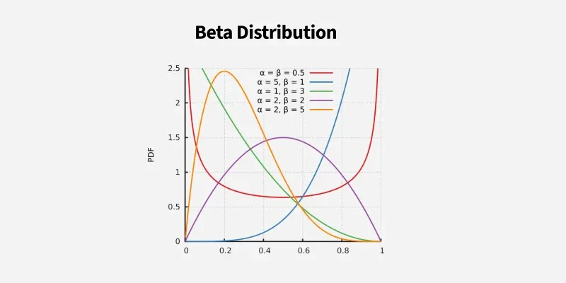
Beta Distribution
5. **Gamma Distribution
The Gamma distribution models the total time needed for multiple independent events to happen. It extends the exponential distribution to cover several tasks or events. For example, estimating the total time to finish three project tasks with varying durations.
- Models total time for multiple events
- Shape parameter (κ) controls event count
- Scale parameter (θ) controls event duration
**PDF Formula:
f(x) = \frac{x^{k-1} e^{-x/\theta}}{\theta^k \Gamma(k)}, \quad x \ge 0

gamma distributions
6. **Chi-Square Distribution
The Chi-Square distribution is used in hypothesis testing to check relationships between categorical variables. For example, testing if gender affects preference for coffee or tea. It helps determine if observed differences are due to chance.
- Used for testing independence between categories
- Works with contingency tables
- Degrees of freedom depend on number of categories
**PDF Formula:
f(x) = \frac{1}{2^{k/2}\Gamma(k/2)} x^{k/2-1} e^{-x/2}
Where:
- k = degrees of freedom

Chi-Square Distributions
7. **Log-Normal Distribution
The Log-Normal distribution models data that grows multiplicatively over time, like stock prices or income. If the logarithm of the data is normally distributed, the original data follows a log-normal distribution. It only models positive values.
- Models multiplicative growth processes
- Data can’t be negative
- Commonly used for stock prices and incomes
**PDF Formula:
f(x) = \frac{1}{x\sigma\sqrt{2\pi}} \exp\left(-\frac{(\ln x - \mu)^2}{2\sigma^2}\right)

Log Normal Distribution
Comparison of Probability Distributions
| Distributions | Key Features | Usage |
|---|---|---|
| Normal Distributions | This is used to adjust data to make it easier to analyze and to find unusual values like errors or outliers. | Used for feature scaling , model assumptions and anomaly detection |
| ExponentialDistributions | It measures how long it takes for something to happen like waiting for an event. | Helps to predict when a server might crash or how long it will take for customers to arrive at a store. |
| Uniform Distributions | In this every possible outcome is equally likely; no outcome is more likely than another. | It is used for picking random samples from a group. |
| Beta Distributions | Helps us to update our guesses about chances based on new information. | This is useful for A/B testing (comparing two options) and figuring out how often people click on links. |
| Gamma Distributions | Gamma measures the total time takes for several events to happen one after another. | Helps to predict when systems might fail and assess risks in various situations. |
| Chi-Square Distributions | It checks if there is a relationship between different categories of data. | helps in analyzing customer survey results to see if different groups have different opinions or behaviors. |
| Log-Normal Distributions | It shows how things grow over time especially when growth happens in steps rather than all at once. | Used for predicting stock prices and understanding how income levels are distributed among people. |
| Binomial Distributions | This models the number of successes in multiple trials. | Useful for determining the probability of a certain number of successes in a fixed number of trials |
| Bernoulli Distributions | Bernoulli models a single trial with two outcomes (success/failure). | Mostly used in quality control to assess pass/fail situations. |
| Poisson Distributions | It find the number of events occurring in a fixed interval of time or space. | Helps to predict the number of customer arrivals at a store during an hour. |
| Geometric Distributions | It helps to find number of trials until the first success occurs. | Useful for understanding how many attempts it takes before achieving the first success e.g., how many times you need to flip a coin before getting heads. |