What is Gradient Descent (original) (raw)
Last Updated : 17 Jan, 2026
Gradient Descent is an iterative optimization algorithm used to minimize a cost function by adjusting model parameters in the direction of the steepest descent of the function’s gradient. In simple terms, it finds the optimal values of weights and biases by gradually reducing the error between predicted and actual outputs.
**For example:
Gradient Descent
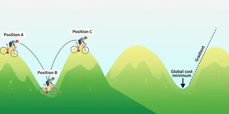
Suppose you're at the top of a hill and your goal is to find the lowest point in the valley. You can't see the entire valley from the top, but you can feel the slope under your feet.
- **Start at the Top: You begin at the top of the hill (this is like starting with random guesses for the model's parameters).
- **Feel the Slope: You look around to find out which direction the ground is sloping down. This is like calculating the gradient, which tells you the steepest way downhill.
- **Take a Step Down: Move in the direction where the slope is steepest (this is adjusting the model's parameters). The bigger the slope, the bigger the step you take.
- **Repeat: You keep repeating the process feeling the slope and moving downhill until you reach the bottom of the valley (this is when the model has learned and minimized the error).
The key idea is that, just like walking down a hill, Gradient Descent moves towards the "bottom" or minimum of the loss function, which represents the error in predictions.
Moving in opposite direction of the gradient allows the algorithm to gradually descend towards lower values of the function and eventually reaching to the minimum of the function. These gradients guide the updates ensuring convergence towards the optimal parameter values. Gradual steps used in descent is done by defining learning rate.
What is Learning Rate?
Learning rate is a important hyperparameter in gradient descent that controls how big or small the steps should be when going downwards in gradient for updating models parameters. It is essential to determines how quickly or slowly the algorithm converges toward minimum of cost function.
**1. If Learning rate is too small: The algorithm will take tiny steps during iteration and converge very slowly. This can significantly increases training time and computational cost especially for large datasets.
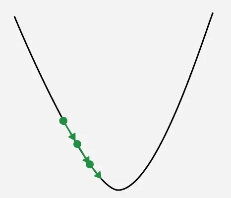
Learning rate with small steps
**2. If Learning rate is too big: The algorithm may take huge steps leading overshooting the minimum of cost function without settling. It fail to converge causing the algorithm to oscillate. This process is termed as exploding gradient problem.
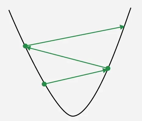
Learning rate with big steps
In image we can see point got oscillated from right to left with converging to minimum gradient value.
To address these problems we have some technique that can be used:
- **Weights Regularzations: The initialization of weights can be adjusted to ensure that they are in an appropriate range. Using a different activation function such as the Rectified Linear Unit (ReLU) can help us to mitigate the vanishing gradient problem.
- **Gradient clipping: Restrict the gradients to a predefined range to prevent them from becoming excessively large or small.
- **Batch normalization: It can also help to address these problems by normalizing the input of each layer to prevent activation function from saturating and hence reducing vanishing and exploding gradient problems.
Choosing right learning rate can leads to fast and stable convergence improving the efficiency of the training process but sometimes vanishing and exploding gradient problem is unavoidable and to address these we have some techniques that we will discuss further in the article.
Mathematics Behind Gradient Descent
For simplicity let's consider a linear regression model with a single input feature x and target y. The loss function (or cost function) for a single data point is defined as the Mean Squared Error (MSE):
J(w, b) = \frac{1}{n} \sum_{i=1}^{n} \left( y_p - y \right)^2
Here:
- y_p = x \cdot w + b: The predicted value.
- w: Weight (slope of the line).
- b: Bias (intercept).
- n: Number of data points.
To optimize the model parameters w, we compute the gradient of the loss function with respect to w. This process involves taking the partial derivatives of J(w,b).
The gradient with respect to w is:
\frac{\partial J(w, b)}{\partial w} = \frac{\partial}{\partial w} \left[ \frac{1}{n} \sum_{i=1}^{n} \left( y_p - y \right)^2 \right]
\frac{\partial J(w, b)}{\partial w} = \frac{2}{n} \sum_{i=1}^{n} (y_p - y) \cdot \frac{\partial}{\partial w} \left( y_p - y \right)
substitute y_p = x \cdot w + b: \frac{\partial J(w, b)}{\partial w} = \frac{2}{n} \sum_{i=1}^{n} (y_p - y) \cdot \frac{\partial}{\partial w} \left( x \cdot w + b - y \right)
**Final Gradient with respect to w:
\frac{\partial J(w, b)}{\partial w} = \frac{2}{n} \sum_{i=1}^{n} (y_p - y) \cdot x
**Gradient Descent Update:
Once the gradients are calculated we update the parameters w in the direction opposite to the gradient (to minimize the loss function):
1. For positive gradient:
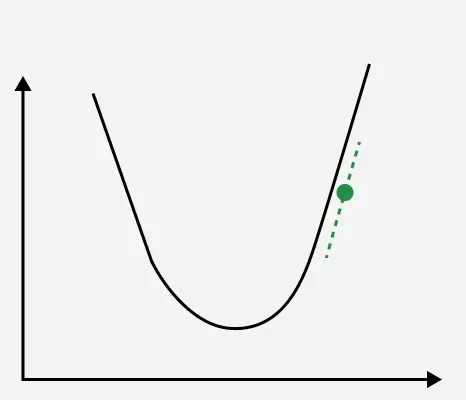
Gradient descent
w = w - \gamma \cdot \frac{\partial J(w, b)}{\partial w}
Here:
- γ: Learning rate (step size for each update).
- ∂w\frac{\partial J(w, b)}{\partial w}: Gradients with respect to w.
Since the gradient is positive subtracting it effectively decreasesw and hence reducing cost function.
2. For Negative Gradient:
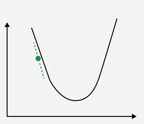
Gradient descent
Since the gradient is negative subtracting it effectively increases w so here we add it to reduce cost function.
Working of Gradient Descent
- **Step 1 we first initialize the parameters of the model randomly
- **Step 2 Compute the gradient of the cost function with respect to each parameter. It involves making partial differentiation of cost function with respect to the parameters.
- **Step 3 Update the parameters of the model by taking steps in the opposite direction of the model. Here we choose a hyperparameter learning rate which is denoted by γ. It helps in deciding the step size of the gradient.
- **Step 4 Repeat steps 2 and 3 iteratively to get the best parameter for the defined model.
Gradient Descent
This animation shows iterative process of gradient descent as it traverses the 3D convex surface of cost function. Each step represents adjustment of model parameters to minimize the loss. It illustrates how the algorithm moves in opposite direction of descent to converge
Implementing Gradient Descent
1. Import libraries: numpy, matplotlib, load_diabetes, StandardScaler.
2. Load diabetes dataset and select BMI feature (X) with target (y).
3. Scale BMI feature using StandardScaler for better gradient descent performance.
4. Initialize parameters: slope m=0, intercept c=0, learning rate 0.05, iterations 1000.
5. Run gradient descent loop:
- Predict values: y_pred = m*X_scaled + c.
- Compute error and Mean Squared Error (MSE).
- Calculate gradients (dm, dc) and update m and c.
- Track loss in loss_history.
- Print progress every 100 iterations. Python `
import numpy as np import matplotlib.pyplot as plt from sklearn.datasets import load_diabetes from sklearn.preprocessing import StandardScaler
diabetes = load_diabetes() X = diabetes.data[:, [2]] y = diabetes.target scaler = StandardScaler() X_scaled = scaler.fit_transform(X) m, c = 0.0, 0.0 learning_rate = 0.05 iterations = 1000 loss_history = []
for i in range(iterations): y_pred = m * X_scaled.flatten() + c error = y_pred - y
loss = np.mean(error ** 2)
loss_history.append(loss)
dm = (2 / len(X_scaled)) * np.dot(error, X_scaled.flatten())
dc = (2 / len(X_scaled)) * np.sum(error)
m -= learning_rate * dm
c -= learning_rate * dc

if i % 100 == 0:
    print(f"Iteration {i}: Loss={loss:.4f}, m={m:.4f}, c={c:.4f}")
print("\nFinal parameters:") print(f"Slope (m): {m:.4f}, Intercept (c): {c:.4f}")
plt.scatter(X_scaled, y, alpha=0.5, label="Real Data") plt.plot(X_scaled, m * X_scaled.flatten() + c, color='red', linewidth=2, label="Fitted Line") plt.xlabel("BMI (scaled)") plt.ylabel("Diabetes Progression") plt.legend() plt.show()
plt.plot(loss_history) plt.xlabel("Iterations") plt.ylabel("Loss (MSE)") plt.title("Loss Curve on Diabetes Dataset") plt.show()
`
**Output:
Different Variants of Gradient Descent
Types of gradient descent are:
- **Batch Gradient Descent: Batch Gradient Descent computes gradients using the entire dataset in each iteration.
- **Stochastic Gradient Descent (SGD): SGD uses one data point per iteration to compute gradients, making it faster.
- **Mini-batch Gradient Descent: Mini-batch Gradient Descent combines batch and SGD by using small batches of data for updates.
- **Momentum-based Gradient Descent: Momentum-based Gradient Descent speeds up convergence by adding a fraction of the previous gradient to the current update.
- **Adagrad: Adagrad adjusts learning rates based on the historical magnitude of gradients.
- **RMSprop: RMSprop is similar to Adagrad but uses a moving average of squared gradients for learning rate adjustments.
- **Adam: Adam combines Momentum, Adagrad and RMSprop by using moving averages of gradients and squared gradients.
For understand their explanation and use-cases, please refer : Types of Gradient Descent.
**Advantages
- **Flexibility: It can be used with various cost functions and can handle non-linear regression problems.
- **Scalability: It is scalable to large datasets since it updates the parameters for each training example one at a time.
- **Convergence: It can converge to global minimum of the cost function provided that the learning rate is set appropriately.
**Disadvantages
- **Sensitivity to Learning Rate: The choice of learning rate is important in gradient descent as it can lead to vanishing or exploding gradient problem.
- **Sensitivity to initialization: It can be sensitive to the initialization of the models parameters which can affect the convergence and the quality of the solution.
- **Local Minima: It can get stuck in local minima, if the cost function has multiple local minima.
- **Time-consuming: It can be time-consuming especially when dealing with large datasets.