Sparse Autoencoders in Deep Learning (original) (raw)
Last Updated : 27 Nov, 2025
To learn efficient data representations with minimal redundancy, Sparse Autoencoders play an important role in deep learning. They are a special type of autoencoder that introduces a sparsity constraint on the hidden layer, forcing only a few neurons to activate at a time.
- Restricts hidden layer activation so the network focuses only on the most informative features.
- Prevents the autoencoder from overfitting or copying inputs directly.
- Helps extract meaningful structure from high-dimensional data.
- The sparsity is typically controlled through regularization techniques like L1 penalty or KL divergence.
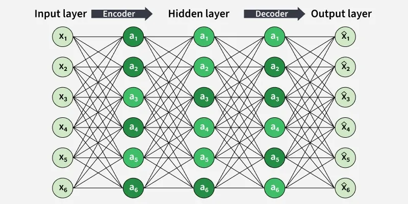
Sparse Auto Encoder
The diagram shows a sparse autoencoder with an encoder-decoder structure, where the hidden layer learns a compressed internal representation by keeping most hidden units inactive (sparse).
Importance of Sparse Autoencoders
Sparse autoencoders are useful for learning compact and meaningful representations of data without supervision.
- **Feature Learning: Extracts important features from unlabeled data for tasks like classification and clustering.
- **Dimensionality Reduction: Compresses high dimensional data while preserving essential information.
- **Anomaly Detection: Identifies unusual inputs that deviate from learned patterns.
- **Denoising: Reconstructs clean data from noisy inputs.
- **Pretraining Networks: Provides a strong weight initialization for deep networks.
- **Interpretable Representations: Sparse activations highlight the most informative features.
How it Works
Sparse autoencoders combine an encoder, decoder and sparsity constrained loss function to learn compact meaningful representations. The loss function used is:
L = \|X - \hat{X}\|^2 + \lambda \cdot \text{Penalty}(s)
**where
- X: Input data
- \hat{X}: Reconstructed output
- \lambda: Regularization parameter
- \text{Penalty}(s): A function penalizing deviations from sparsity
Working:
- Encoder compresses the input into a low dimensional latent representation.
- Decoder reconstructs the input from the encoded features.
- Sparsity Constraint ensures only a small number of hidden neurons activate for each input.
Methods to Enforce Sparsity
Sparsity is enforced to ensure the autoencoder learns high level features by activating only a small subset of neurons
- **L1 Regularization****:** Applies a penalty proportional to the absolute activations or weights, encouraging the network to use fewer neurons.
- **KL Divergence****:** Measures how far the average activation deviates from the target sparsity level, ensuring that only a subset of neurons activates at a time.
- **Sparsity Proportion: Defines the desired activation frequency of hidden units across training samples.
How Sparse Autoencoders Are Trained
Training a sparse autoencoder follows the same workflow as a standard autoencoder but includes an additional step to enforce sparsity on the hidden layer:
**1. Initialization: The network weights are initialized randomly or using pre-trained models to provide a stable starting point.
**2. Forward Pass: Input data is passed through the encoder to obtain the latent (compressed) representation and then through the decoder to reconstruct the original input.
**3. Loss Calculation: The total loss combines:
- **Reconstruction error: MSE between X and \hat{X}
- **Sparsity penalty: Uses KL Divergence or L1 regularization to keep most hidden units inactive.
**4. Backpropagation and Optimization: Gradients are computed from the combined loss and used to update the network weights, ensuring the model learns both accurate reconstruction and sparse feature representations.
Step-By-Step Implementation
Here builds a Sparse Autoencoder using TensorFlow and Keras to learn compressed, sparse feature representations. The network is designed to learn compressed and sparse feature representations of the input data, enabling efficient encoding while retaining important information.
Step 1: Import Libraries
Here we will import tensorflow and keras, numpy and matplotlib.
Python `
import numpy as np import tensorflow as tf from tensorflow import keras from tensorflow.keras import layers import matplotlib.pyplot as plt
`
Step 2: Load and Preprocess Dataset
- MNIST dataset is loaded.
- 28×28 images are flattened into 784 dim vectors.
- Pixel values are normalized to the range [0, 1]. Python `
(x_train, _), (x_test, _) = keras.datasets.mnist.load_data()
x_train = x_train.reshape((x_train.shape[0], -1)).astype('float32') / 255.0 x_test = x_test.reshape((x_test.shape[0], -1)).astype('float32') / 255.0
`
Step 3: Define Model Parameters
- **input_dim: number of pixels (784).
- **hidden_dim: size of the bottleneck (sparse layer).
- **sparsity_level: desired average activation (ρ = 0.05).
- **lambda_sparse: weight applied to sparsity penalty. Python `
input_dim = 784 hidden_dim = 64 sparsity_level = 0.05 lambda_sparse = 0.1
`
Step 4: Build the Autoencoder Model
- **layers.Input****:** Defines the input layer with the shape of the flattened images.
- **layers.Dense (encoded): Creates the hidden layer with ReLU activation to compress input into a sparse representation.
- **layers.Dense (decoded): Creates the output layer with sigmoid activation to reconstruct the original input.
- **keras.Model (autoencoder): Combines input and decoded output to form the full autoencoder model.
- **keras.Model (encoder): Defines a separate model from input to encoded layer for extracting compressed features. Python `
inputs = layers.Input(shape=(input_dim,)) encoded = layers.Dense(hidden_dim, activation='relu')(inputs) decoded = layers.Dense(input_dim, activation='sigmoid')(encoded)
autoencoder = keras.Model(inputs, decoded) encoder = keras.Model(inputs, encoded)
`
Step 5: Define Sparse Loss Function
- Computes normal reconstruction error using MSE.
- Extracts hidden-layer activations from the encoder.
- Computes mean activation per unit.
- Uses KL divergence to enforce sparsity. Python `
def sparse_loss(y_true, y_pred): mse_loss = tf.reduce_mean(keras.losses.MeanSquaredError()(y_true, y_pred))
hidden_layer_output = encoder(y_true)
mean_activation = tf.reduce_mean(hidden_layer_output, axis=0)

kl_divergence = tf.reduce_sum(
    sparsity_level * tf.math.log(sparsity_level / (mean_activation + 1e-10)) +
    (1 - sparsity_level) * tf.math.log((1 - sparsity_level) / (1 - mean_activation + 1e-10))
)

return mse_loss + lambda_sparse * kl_divergence
`
Step 6: Compile the Autoencoder
- Uses Adam optimizer for fast convergence.
- Uses custom sparse loss function. Python `
autoencoder.compile(optimizer='adam', loss=sparse_loss)
`
Step 7: Train the Autoencoder
- **autoencoder.fit: Trains the autoencoder model.
- **epochs: Runs the training for 50 complete passes over the dataset.
- **batch_size: Updates model weights after every 256 samples.
- **shuffle: Shuffles the training data before each epoch to improve learning. Python `
history = autoencoder.fit( x_train, x_train, epochs=50, batch_size=256, shuffle=True )
`
Step 8: Reconstruct Test Images
Autoencoder predicts reconstructed images from test inputs.
Python `
reconstructed = autoencoder.predict(x_test)
`
Step 9: Visualize Original vs Reconstructed Images
- First row shows original images.
- Second row shows reconstructed versions. Python `
n = 10 plt.figure(figsize=(20, 4))
for i in range(n): ax = plt.subplot(2, n, i + 1) plt.imshow(x_test[i].reshape(28, 28), cmap='gray') plt.title("Original") plt.axis('off')
ax = plt.subplot(2, n, i + 1 + n)
plt.imshow(reconstructed[i].reshape(28, 28), cmap='gray')
plt.title("Reconstructed")
plt.axis('off')
plt.show()
`
**Output:
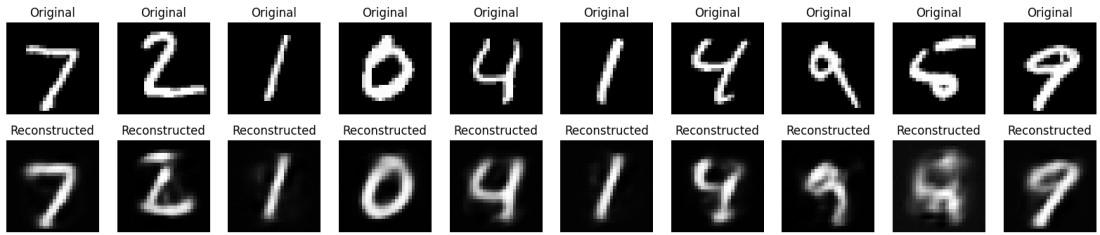
Reconstructed Images
Step 10: Visualize Encoded Feature Space
Computes 2D encoded representations of the input data.
Python `
encoded_outputs = encoder.predict(x_train)
plt.figure(figsize=(10, 8)) plt.scatter(encoded_outputs[:, 0], encoded_outputs[:, 1], s=2) plt.title("Encoded Feature Space") plt.xlabel("Dimension 1") plt.ylabel("Dimension 2") plt.show()
`
**Output:
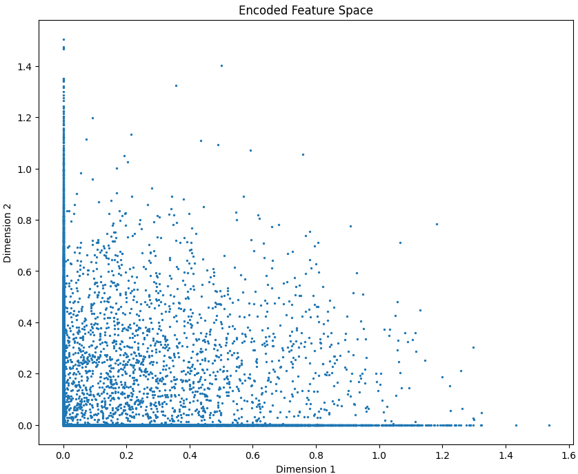
Encoded Feature Space
The scatter plot visualizes the 2-dimensional encoded feature space learned by the autoencoder. It shows how input samples cluster after compression, with many points near zero, indicating sparse activations typical of sparse autoencoders.
Step 10: Analyze Encoded Representations
- Extract hidden features from encoder.
- Plot mean activation to verify sparsity. Python `
encoded_outputs = encoder.predict(x_train) mean_activation = np.mean(encoded_outputs, axis=0)
plt.figure(figsize=(10, 4)) plt.bar(range(len(mean_activation)), mean_activation) plt.title("Mean Activation of Hidden Units") plt.xlabel("Hidden Unit Index") plt.ylabel("Mean Activation") plt.show()
`
**Output:
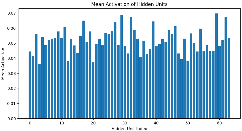
Mean Activation
This plot displays the average activation of each hidden neuron in the sparse autoencoder, showing how frequently each unit is used. The lower and uneven activation values indicate that only a few neurons fire strongly while most remain inactive, confirming that the model has learned sparse and specialized feature detectors as intended.
You can download full code from here.
Applications
- **Feature Extraction: Learns important features from raw data for tasks like classification and clustering.
- **Dimensionality Reduction: Reduces high dimensional data while preserving key information.
- **Anomaly Detection: Detects unusual patterns by identifying inputs that cannot be well reconstructed.
- **Image Denoising: Removes noise from images by learning the underlying clean representation.
- **Pretraining for Deep Networks: Initializes weights in deep networks to improve convergence and performance.
Advantages
- **Efficient Feature Learning: Learns compact and meaningful representations of data.
- **Reduces Overfitting: Sparsity constraint prevents the network from memorizing data.
- **Handles High Dimensional Data: Can compress large input data effectively.
- **Improves Downstream Tasks: Enhances performance in classification, clustering and anomaly detection.
- **Flexible Architecture: Can be combined with other models or used for pretraining deep networks.
Challenges
- **Choosing Sparsity Level: Setting an appropriate sparsity target can be tricky and impacts performance.
- **Computational Complexity: Training can be slow for large datasets or deep architectures.
- **Risk of Underfitting: Too much sparsity may cause the model to miss important features.
- **Hyperparameter Tuning: Requires careful tuning of learning rate, hidden units and regularization.
- **Sensitive to Initialization: Poor weight initialization can lead to vanishing/exploding gradients.