Training and Validation Loss in Deep Learning (original) (raw)

Last Updated : 27 Nov, 2025

Training loss measures how well the model learns from the training data during training. Validation loss shows how well the trained model performs on unseen data, helping detect overfitting.

Training Loss

Training Loss is a metric that measures how well a deep learning model is performing on the training dataset. During training the model makes predictions and compares them with the actual target values. The loss function then calculates the error between these predicted outputs and the true labels.

Training loss is computed after each forward pass and backward pass . The training loss can be expressed as:

\text{Loss} = \frac{1}{N} \sum_{i=1}^{N} L(y_i, \hat{y}_i)

Where:

• N: Total number of training examples
• y_i: True label
• \hat{y}_i​: Predicted output
• L: Chosen loss function

A lower training loss means the model is learning well, whereas a high training loss often indicates underfitting or difficulty in learning patterns.

Validation Loss

Validation loss is a metric that evaluates a deep learning model’s performance on a validation dataset (set of data that the model has never seen during training). Validation loss is computed after each epoch during training

\text{Validation Loss} = \frac{1}{M} \sum_{i=1}^{M} L(y_i^{\text{val}}, \hat{y}_i^{\text{val}})

where

• M: number of validation examples
• y_i^{\text{val}}: true label of the i^{\text{th}} validation example
• \hat{y}_i^{\text{val}}: predicted output for the i^{\text{th}} validation example

Importance of Monitoring Both Losses

• **Detect Overfitting: Training loss decreases but validation loss increases indicating the model is memorizing the training data.
• **Detect Underfitting: Both losses remain high, showing the model is too simple or not learning patterns well.
• **Hyperparameter Tuning: Loss trends help adjust learning rate, batch size, architecture and regularization.
• **Generalization: Validation loss reflects how well the model performs on unseen real world data.
• **Optimize Training Process: Monitoring both losses supports decisions like early stopping and learning rate scheduling.

Step-By-Step Implementation

Here we train a simple CNN on the Fashion MNIST dataset, monitor training and validation loss and plot the loss curves.

Step 1: Import Libraries

Here we will import TensorFlow, Keras and Matplotlib.

Python `

import tensorflow as tf from tensorflow.keras.datasets import fashion_mnist from tensorflow.keras.models import Sequential from tensorflow.keras.layers import Conv2D, MaxPooling2D, Flatten, Dense, Dropout from tensorflow.keras.utils import to_categorical import matplotlib.pyplot as plt

`

Step 2: Load and Preprocess Dataset

• Loads Fashion MNIST images and labels into training and testing sets.
• Reshapes images for CNN input.
• Normalizes pixel values to the range [0, 1].
• Converts integer labels into one-hot encoded. Python `

(X_train, y_train), (X_test, y_test) = fashion_mnist.load_data()

X_train = X_train.reshape(-1, 28, 28, 1) / 255.0 X_test = X_test.reshape(-1, 28, 28, 1) / 255.0

y_train = to_categorical(y_train, 10) y_test = to_categorical(y_test, 10)

`

Step 3: Build CNN Model

• **Sequential model****:** Stack layers.
• **Conv2D****:** Extracts local features from images.
• **MaxPooling2D****:** Reduces spatial size and computational cost.
• **Flatten()****:** Converts 2D feature maps into a 1D vector.
• **Dense()****:** Fully connected layer to learn complex relationships.
• **Dropout()****:** Randomly drops neurons to reduce overfitting. Python `

model = Sequential([ Conv2D(32, (3,3), activation='relu', input_shape=(28,28,1)), MaxPooling2D((2,2)), Conv2D(64, (3,3), activation='relu'), MaxPooling2D((2,2)), Flatten(), Dense(128, activation='relu'), Dropout(0.5), Dense(10, activation='softmax') ])

`

Step 4: Compile Model

• **Adam Optimizer****:** Adaptive optimizer that adjusts learning rates for faster and efficient training.
• **Categorical Cross-Entropy Loss: Ideal for multi-class classification tasks, penalizes wrong predictions.
• **Accuracy Metric: Tracks how many predictions match the true labels during training and validation. Python `

model.compile(optimizer='adam', loss='categorical_crossentropy', metrics=['accuracy'])

`

Step 5: Train Model with Validation Split

• Trains the model for 15 epochs.
• Uses 64 images per batch.
• Reserves 20% of training data as validation set to measure generalization.
• Stores loss and accuracy values in history for later plotting. Python `

history = model.fit(X_train, y_train, epochs=15, batch_size=64, validation_split=0.2)

`

**Output:

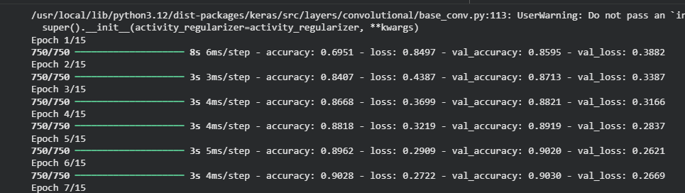
Traning

Step 6: Plot Training and Validation Loss

• Creates a loss graph using matplotlib.
• Plots training loss across epochs.
• Plots validation loss on the same graph for comparison.
• Helps identify overfitting, underfitting, or stable training. Python `

plt.figure(figsize=(8,5)) plt.plot(history.history['loss'], label='Training Loss') plt.plot(history.history['val_loss'], label='Validation Loss') plt.title('Training vs Validation Loss (CNN)') plt.xlabel('Epochs') plt.ylabel('Loss') plt.legend() plt.show()

`

**Output:

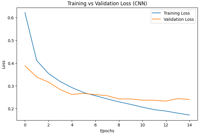
Training vs Validation

The graph shows that both training and validation loss decrease steadily over epochs indicating effective learning. The gap between the curves remains small, showing the model is not overfitting and generalizes well to unseen data.

You can download full code from here.

Loss Functions for Model Training

1. **Mean Squared Error****:** MSE measures the average squared difference between predicted and actual values in regression tasks.
2. **Mean Absolute Error****:** MAE calculates the average absolute difference between predicted outputs and true values.
3. **Cross-Entropy Loss****:** Cross-Entropy Loss measures how well the predicted probability distribution matches the true class labels in classification tasks.
4. **Huber Loss****:** Huber Loss combines MSE and MAE to provide a balanced, outlier-resistant error measure.

Patterns in Loss Curves

• **Both Training and Validation Loss Decrease: The model is learning well and generalizing properly. This indicates healthy training, and no major changes are needed unless the curves stop improving.
• **Training Loss Decreases Validation Loss Increases: The model is overfitting and memorizing the training data.
• **Both Training and Validation Loss Remain High: The model is underfitting and failing to learn patterns.
• **Validation Loss Lower than Training Loss: validation loss is slightly lower due to regularization or easier validation samples. This is usually not a problem if the difference is small.
• **Sudden Spikes in Validation Loss: Occasional spikes in validation loss may occur due to noisy data or a high learning rate

**Factors That Affect Loss Values

Several factors influence how training and validation loss behave during model training.

• **Learning Rate: A high learning rate causes unstable loss, a low learning rate slows down convergence.
• **Batch Size: Small batch sizes add noise, while large batches produce smoother but slower updates.
• **Model Complexity: Too simple models underfit, too complex models overfit.
• **Quality of Data: Noisy, unbalanced or poor-quality data increases both training and validation loss.
• **Weight Initialization: Poor initialization may lead to exploding/vanishing gradients.

Techniques to Reduce Training and Validation Loss

• **Improve Data Preprocessing: Normalize, clean and structure data for faster and more accurate learning.
• **Better or Deeper Architectures: Add layers, filters or skip connections to capture complex patterns.
• **Advanced Optimizers: Adam, RMSProp and AdamW stabilize and speed up convergence.
• **L1/L2 Regularization: Penalizes large weights to prevent overfitting.
• **Dropout: Randomly disables neurons to reduce reliance on specific features.
• **Batch Normalization: Stabilizes training and reduces overfitting by normalizing layer inputs.
• **Data Augmentation: Creates varied training samples to improve generalization.
• **Early Stopping: Halts training when validation loss stops improving to avoid overfitting.