Split Cells in Excel (original) (raw)
Last Updated : 18 Mar, 2026
Splitting cells in Excel can simplify data management, especially when dealing with combined information in a single column or cell. Whether you’re separating names, dates, or other data points, understanding how to split cells in Excel is essential for better organization and clarity.
Excel provides multiple methods to achieve this:
- Text to Columns for quick splitting based on delimiters.
- Fixed Width for precise splits at character positions.
- Formulas for customizable splitting based on patterns.
- Flash Fill for automated splitting based on user-defined examples.
- Power Query for advanced and scalable data transformations.
In the below data set, Column A has both Products and categories combined with a space delimiter.

Dataset
Split Cells in Excel Using Text to Columns
The Text to Columns feature is a simple yet powerful tool for divide cells based on delimiters or fixed widths.
Method 1. Split Using Delimiters
Follow the below steps to separate Cells in Excel without losing data using text to column option:
**Step 1: Select the Data Range
Select the entire data set in which you want to break up cells in excel. Here we have selected A1: A11.
**Step 2: Go to the Data Tab
Go to “Data” tab, Click “Text to Columns”, to pop up Convert Text to Columns Wizard.
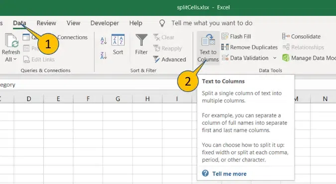
Go to Data Tab >> Click on "Text to Columns"
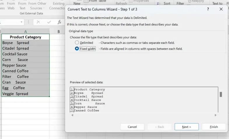
**Step 3: Select “Delimited” and Press “Next”
Select Delimited and click Next.
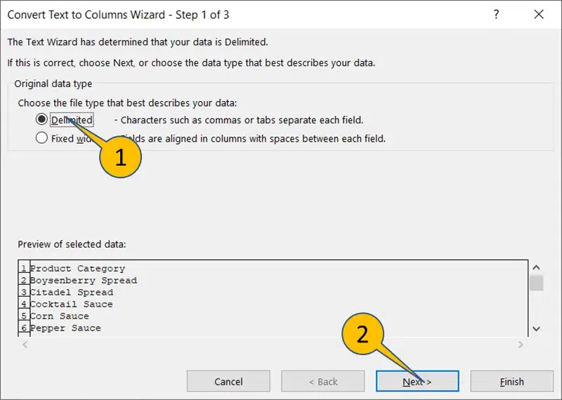
Select “Delimited” >> Press “Next”
**Step 4: Check “Space” and Press “Next”
Check Space as the delimiter to split the names at spaces. Click Next.
**Note: You can Choose other functions also such as Comma, Tab etc. to divide the cell in excel.
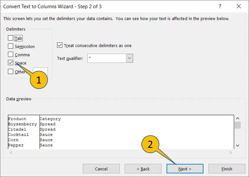
Check Space >> Press Next
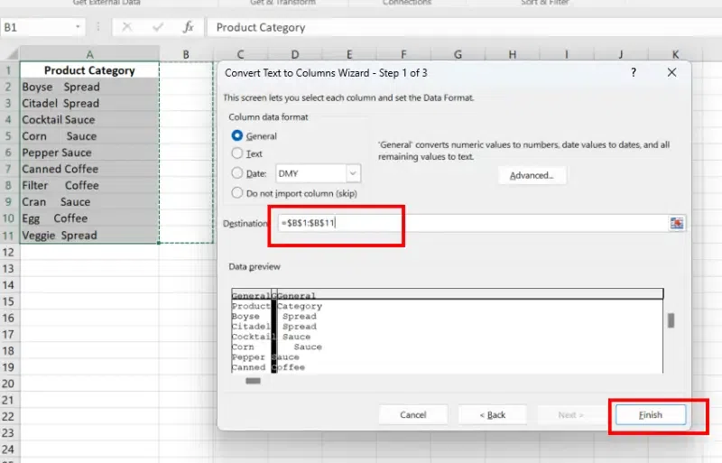
**Step 5: Change Destination and Press Next
Enter your Destination and Press “Finish” .Here we have selected BBB1.
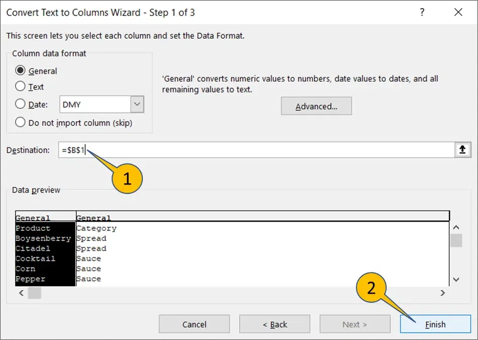
Enter Destination >> Click "Ok"
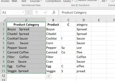
**Step 6: Preview the Excel Split Cell

Split Cells Achieved
Method 2: Split Using Fixed Width
The Fixed Width option in Excel allows you to split text in a cell at specific character positions. You can use this way to split a single cell into multiple columns. Follow these steps to know how to divide cells in excel into multiple columns:
**Step 1: Select the Data Range
Highlight the cells containing the text you want to split.
**Step 2: Open the Text to Columns Wizard
- Go to the Data tab in the toolbar.
- Click on Text to Columns.
**Step 3: Choose Fixed Width
In the wizard, select the Fixed Width option and click Next.
Select Data>>Go to Data Tab>>Fixed Width>>Next
**Step 4: Set Break Lines
Click in the preview window to place break lines where you want the text to split.
Drag thebreak lines to adjust their position if needed.
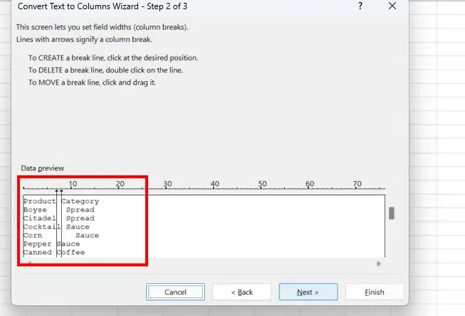
Drag the Break as per your choice and Click next
**Step 5: Select Destination
Choose where the split text should appear. By default, Excel will overwrite the original data unless you select a different destination column.
Select the destination and Click on Finish
**Step 6: Preview Results
Excel will split the data into separate columns based on your specified widths.
Preview Results
**Pro Tip: Always make a backup of your data before using Text to Columns, as it overwrites the original cells by default.
**Split Cells in Excel Using Formulas
Formulas provide flexibility when dealing with inconsistent data formats, such as middle names or extra spaces.
**Common Formulas for Splitting Cells:
**Extract First Word:
=LEFT(A2, FIND(" ", A2) - 1)
**Extract Last Word:
=RIGHT(A2, LEN(A2) - FIND(" ", A2))
**Extract Middle Name:
=MID(A2, FIND(" ", A2) + 1, FIND(" ", A2, FIND(" ", A2) + 1) - FIND(" ", A2) - 1)
Follow the below steps to Split Cells in Excel Using Formulas:
Type Header text “Product” and “Category” to cells B1 and C1 respectively
**Step 2: Enter Formula
Write the below formula in cell B2 to split the first word (Product)
=LEFT(A2,FIND(" ",A2)-1)
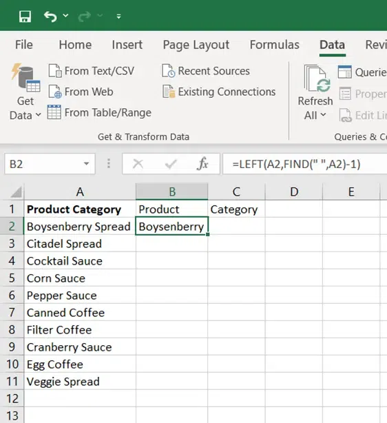
Type Header
**Step 3: Fill the formula in cells B2:B11
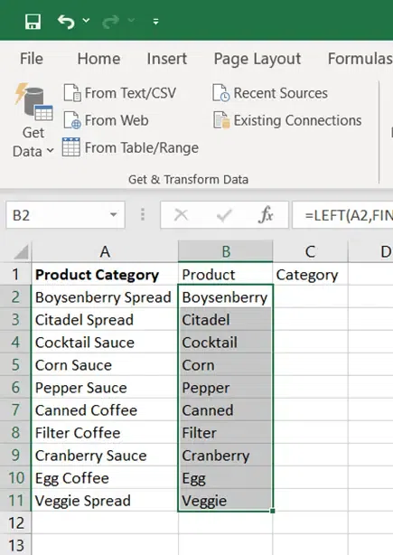
Enter Formula
**Step 4: Enter Formula in C2
Write the below formula in cell C2 to split the last word (Category)
**=RIGHT(A2,LEN(A2)-FIND(" ",A2))

Write Formula in C2
**Step 5: Fill the formula in cells C2:C11

Fill the Formula from C2:C11
Split Cells in Excel Using Flash Fill - 2 Methods
Excel cell splitting using basic patterns is fairly simple to utilize. It can run in two possible ways:
- In the background
- Triggered manually by the user
Method 1: Background execution
In this, Excel automatically offers ideas after trying to identify trends in the text.
**Step 1: Type the Text Element
Type the text element we want to extract in the first row of the first column (with the source cells on the left). Enter the portion of the text from the second cell that we wish to extract. Flash Fill now takes action and offers suggestions.

Type the text
**Step 2: Press Tab Key
To accept the suggested fill, press the Tab or Enter key.

Enter Key
Method 2: Manual Execution
Now that we've seen how the Flash fill auto-suggests the data, let's have a look at the manual approach as well.

Manual Execution
**Step 1: Type the Text Element
In any single row, type the text element that has to be extracted. In this particular example (Last name)
**Step 2: Go to the Home Tab
Click Home Tab and Fill (dropdown) > Flash Fill, and choose the cells in the range that should have values entered.
.webp)
Go to the Home Tab >> Click on "Fill Tab"
**Pro Tip: Flash Fill works best with consistent data and patterns.
**Split Cells in Excel Using Power Query
Excel's Power Query feature can also be used to divide several cells. It has been natively available since Excel 2016.
Let's start off with adding our data cells into the Power Query editor. The steps to take are listed below,
**Step 1: Go to the Home Tab
Click Data tab and from Table/Range after choosing any cell from the data set
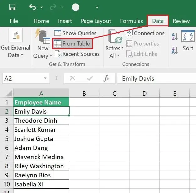
Go to the Data Tab
**Step 2. Click "Ok"
Make sure the "My table has headers" option is checked, and the whole range is selected. Then press OK.
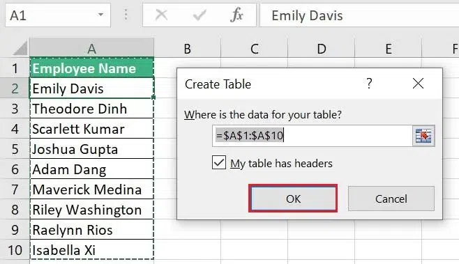
Click "Ok"
**Step 3. Data Visible
All the data will be visible when the Power Query editor opens.
**Step 4. Go to the Home Tab
Select Home > Split Column (drop-down) > By Delimiter from the Power Query ribbon.
.webp)
Go to the Home Tab
**Step 5. Click "Ok"
The Space character and At each occurrence of the delimiter are both suitable choices for our circumstances. Select OK
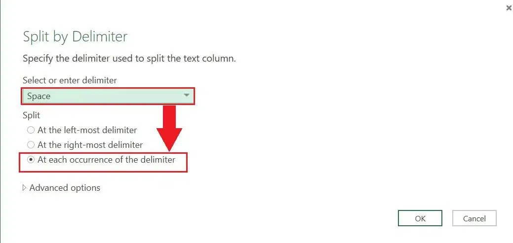
Select "Ok"
**Step 6. Change Heading If necessary
The Employee name column is now divided into two distinct columns in the data preview pane. To change the headings to First name and Last name, double-click the header and make changes respectively.
.webp)
Double Click the header to change
Divide a Cell in Excel in Excel Using Text Functions in Excel
There are many Text Functions in Excel, but we don't need all of them here. A few of them are mentioned below:
- **LEN- Returns the length of a String.
- **RIGHT- Extract a specified number of characters from a String's right end.
- **LEFT- Extract a specified number of characters from a String's left end.
- **FIND- Look for a string inside another string.
- **SEARCH- Return the positions of a string inside another string.
- **MID- Extract a specified number of characters from a String's center.
You can use any combination of the above text Functions to achieve your excel splitting cells.
Enter the Formula =LEFT(A2,SEARCH(" ",A2)-1) in cell B2.
The **SEARCH looks for any space in the customer name and returns its position in the string. Then, the LEFT function extracts the part of the String from the left side, up to the position returned by the SEARCH Function. Now you are done with excel split cell.
Common Use Cases for Splitting Cells in Excel
How to Separate a Cell in Excel
Split names, addresses, or product details for better organization.
How to Bifurcate Data in Excel
Categorize data into Above/Below categories using IF formulas.
How to Divide a Cell in Excel
Use the Fixed Width or Text to Columns option for detailed splitting