Association Rule (original) (raw)
Last Updated : 2 May, 2026
Association rules are a fundamental concept used to find relationships, correlations or patterns within large sets of data items. They describe how often itemsets occur together in transactions and express implications of the form:
X \rightarrow Y
Where X and Y are disjoint sets of items. This rule suggests that when items in X appear, items in Y tend to appear as well. Association rules originated from market basket analysis and help retailers and analysts understand customer behavior by discovering item associations in transaction data. For example, a rule stating
\{ \text{Bread}, \text{Butter} \} \;\rightarrow\; \{ \text{Milk} \}
Indicates that customers who buy bread and butter also tend to buy milk.
Key Components
- **Antecedent (X): The "if" part representing one or more items found in transactions.
- **Consequent (Y): The "then" part, representing the items likely to be purchased when antecedent items appear.
Rules are evaluated based on metrics that quantify their strength and usefulness:
Rule Evaluation Metrics
**1. Support: Fraction of transactions containing the itemsets in both X and Y.
\text{Support}(X \rightarrow Y) = \frac{\text{Number of transactions with } (X \cup Y)}{\text{Total number of transactions}}
Support measures how frequently the combination appears in the data.
**2. Confidence: Probability that transactions with X also include Y.
\text{Confidence}(X \rightarrow Y) = \frac{\text{Support}(X \cup Y)}{\text{Support}(X)}
Confidence measures the reliability of the inference.
**3. Lift: The ratio of observed support to that expected if X and Y were independent.
\text{Lift}(X \rightarrow Y) = \frac{\text{Confidence}(X \rightarrow Y)}{\text{Support}(Y)}
- Lift > 1 implies a positive association — items occur together more than expected.
- Lift = 1 implies independence.
- Lift < 1 implies a negative association.
**Example Transaction Data
| Transaction ID | Items |
|---|---|
| 1 | Bread, Milk |
| 2 | Bread, Diaper, Beer, Eggs |
| 3 | Milk, Diaper, Beer, Coke |
| 4 | Bread, Milk, Diaper, Beer |
| 5 | Bread, Milk, Diaper, Coke |
Considering the rule:
\{ \text{Milk}, \text{Diaper} \} \;\rightarrow\; \{ \text{Beer} \}
**Calculations:
- Support =\frac 2 5 = 0.4
- Confidence = \frac 2 3 \approx 0.67
- Lift = \frac{0.67}{0.6} = 1.11 (positive association)
Implementation
Let's see the working,
Step 1: Install and Import Libraries
We will install and import all the required libraries such as pandas, mixtend, matplotlib, networkx.
Python `
!pip install pandas mlxtend matplotlib seaborn networkx
import pandas as pd from mlxtend.preprocessing import TransactionEncoder from mlxtend.frequent_patterns import apriori, association_rules import matplotlib.pyplot as plt import seaborn as sns import networkx as nx
`
Step 2: Load and Preview Dataset
We will upload the dataset,
Python `
data = pd.read_csv("Groceries_dataset.csv")
print(data.head())
`
**Output:
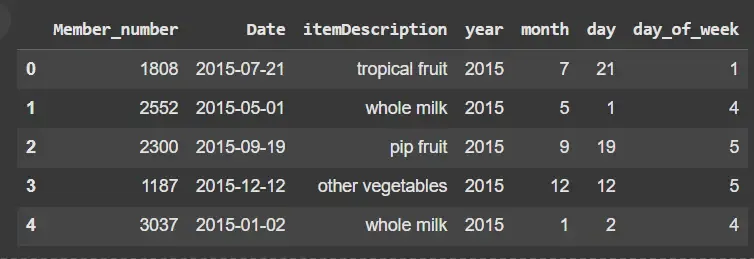
Dataset
Step 3: Prepare Data for Apriori Algorithm
Apriori requires this one-hot encoded format where columns = items and rows = transactions with True/False flags.
Python `
transactions = data.groupby('Member_number')[ 'itemDescription'].apply(list).values.tolist()
te = TransactionEncoder() te_ary = te.fit(transactions).transform(transactions) df = pd.DataFrame(te_ary, columns=te.columns_) df.head()
`
**Output:
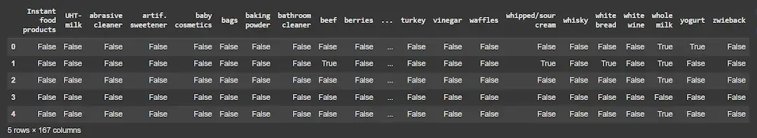
Preparing Data for Apriori Algorithm
Step 4: Generate Frequent Itemsets
We will,
- Finds itemsets appearing in ≥ 1% of all transactions.
- use_colnames=True to keep item names readable. Python `
frequent_itemsets = apriori(df, min_support=0.01, use_colnames=True)
print(frequent_itemsets.head())
`
**Output:
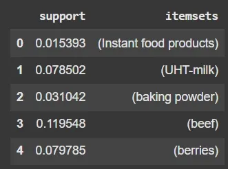
Frequent Itemsets
Step 5: Generate Association Rules
We will,
- Extract rules with confidence ≥ 30%.
- Rules DataFrame includes columns like antecedents, consequents, support, confidence and lift. Python `
rules = association_rules( frequent_itemsets, metric="confidence", min_threshold=0.3)
print(rules.head())
`
**Output:
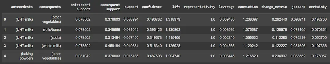
Result
**Step 6: Visualize Top Frequent Items
We will,
- Visualizes the 10 most purchased items.
- Helps understand popular products in the dataset. Python `
item_frequencies = df.sum().sort_values(ascending=False)
plt.figure(figsize=(10, 6)) sns.barplot(x=item_frequencies.head(10).values, y=item_frequencies.head(10).index) plt.title('Top 10 Frequent Items') plt.xlabel('Frequency') plt.ylabel('Items') plt.show()
`
**Output:
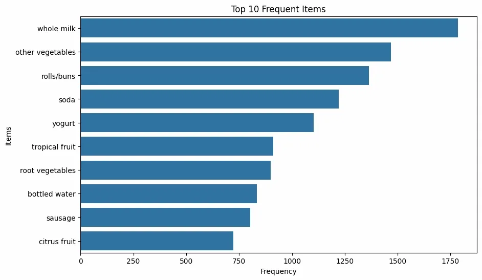
Visualizing Top Frequent Items
Step 7: Scatter Plot of Rules(Support vs Confidence)
Here we will,
- Shows the relationship between support and confidence for rules.
- Color encodes the strength of rules via lift. Python `
plt.figure(figsize=(8, 6)) scatter = plt.scatter(rules['support'], rules['confidence'], c=rules['lift'], cmap='viridis', alpha=0.7) plt.colorbar(scatter, label='Lift') plt.xlabel('Support') plt.ylabel('Confidence') plt.title('Scatter Plot of Association Rules') plt.show()
`
**Output:
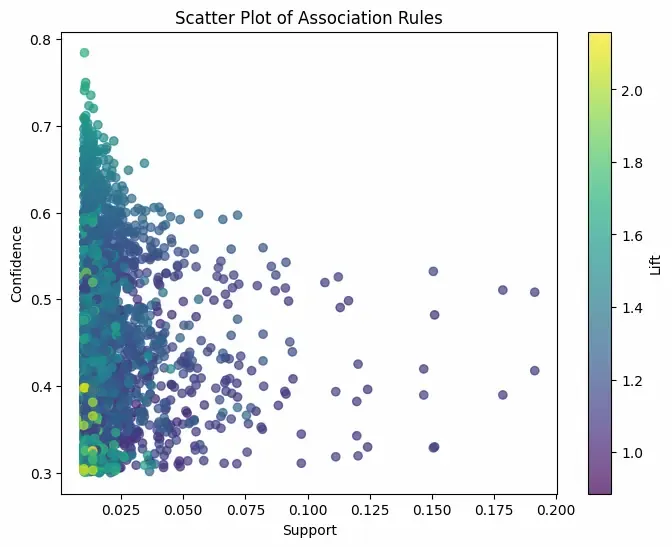
Scatter Plot
Step 8: Heatmap of Confidence for Selected Rules
We will,
- Shows confidence values between top antecedent and consequent itemsets.
- A quick way to identify highly confident rules. Python `
rules['antecedents_str'] = rules['antecedents'].apply( lambda x: ', '.join(list(x))) rules['consequents_str'] = rules['consequents'].apply( lambda x: ', '.join(list(x)))
top_ants = rules.groupby('antecedents_str')['support'].sum().nlargest(10).index top_cons = rules.groupby('consequents_str')['support'].sum().nlargest(10).index
filtered = rules[(rules['antecedents_str'].isin(top_ants)) & (rules['consequents_str'].isin(top_cons))]
heatmap_data = filtered.pivot( index='antecedents_str', columns='consequents_str', values='confidence')
plt.figure(figsize=(12, 8)) sns.heatmap(heatmap_data, annot=True, cmap='YlGnBu', linewidths=0.5, cbar_kws={'label': 'Confidence'}) plt.title('Heatmap of Confidence for Top Association Rules') plt.xlabel('Consequents') plt.ylabel('Antecedents') plt.show()
`
**Output:
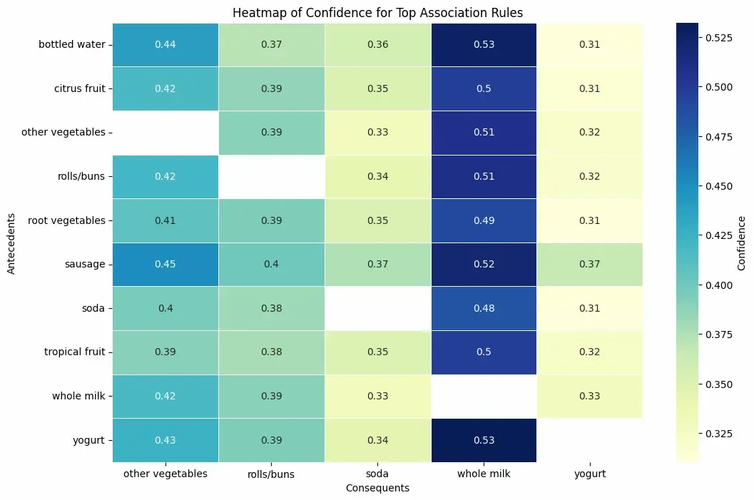
Heatmap
Use Cases
Let's see the use case of Association rule,
- **Market Basket Analysis: Identifies products often bought together to improve store layouts and promotions (e.g., bread and butter).
- **Recommendation Systems: Suggests related items based on buying patterns (e.g., accessories with laptops).
- **Fraud Detection: Detects unusual transaction patterns indicating fraud.
- **Healthcare Analytics: Finds links between symptoms, diseases and treatments (e.g., symptom combinations predicting a disease).
Advantages
- **Interpretable and Easy to Explain: Rules offer clear “if-then” relationships understandable to non-technical stakeholders.
- **Unsupervised Learning: Works well on unlabeled data to find hidden patterns without prior knowledge.
- **Flexible Data Types: Effective on transactional, categorical and binary data.
- **Helps in Feature Engineering: Can be used to create new features for downstream supervised models.
Limitations
- **Large Number of Rules: Can generate many rules, including trivial or redundant ones, making interpretation hard.
- **Support Threshold Sensitivity: High support thresholds miss interesting but infrequent patterns; low thresholds generate too many rules.
- **Not Suitable for Continuous Variables: Requires discretization or binning before use with numerical attributes.
- **Computationally Expensive: Performance degrades on very large or dense datasets due to combinatorial explosion.
- **Statistical Significance: High confidence doesn’t guarantee a meaningful rule; domain knowledge is essential to validate findings.