CatBoost Bayesian optimization (original) (raw)

Last Updated : 23 Jul, 2025

Bayesian optimization is a powerful and efficient technique for hyperparameter tuning of machine learning models and CatBoost is a very popular gradient boosting library which is known for its robust performance in various tasks. When we combine both, Bayesian optimization for CatBoost can offer an effective, optimized, memory and time-efficient approach to find optimal hyperparameter values that can significantly enhance the predictive performance of CatBoost models.

What is CatBoost

CatBoost or Categorical Boosting is a well-known machine learning algorithm developed by Yandex, a Russian multinational IT company. This special boosting algorithm utilizes the gradient boosting framework and is designed to handle categorical features more effectively than traditional gradient boosting algorithms by incorporating several techniques like ordered boosting, oblivious trees, and advanced handling of categorical variables to achieve high performance with minimal hyperparameter tuning. But this hyperparameter tuning can't be done by random guessing which is time-consuming and un-processional way. In this article, we will employ the Bayesian optimization technique to get the best values of hyperparameters then we will visualize the optimization process.

What is Bayesian Optimization

Bayesian optimization is a global optimization technique used to optimize complex and expensive objective functions that are encountered during hyperparameter tuning. Unlike traditional grid search or random search, Bayesian optimization utilizes a probabilistic model to estimate the objective function's behaviour and guide the search process which balances exploration and exploitation to efficiently locate the optimal set of hyperparameters. There are some key benefits listed below:

**Efficiency: Bayesian optimization minimizes the number of model evaluations required to find the best hyperparameters by intelligently selecting hyperparameter combinations that are more likely to yield improved results which greatly reduces the computational cost.
**Global Optimization: Unlike grid search or random search which explores hyperparameters in a deterministic or random manner, Bayesian optimization considers uncertainty and aims to find the global optimum rather than getting stuck in local optima which makes it more accurate for hyperparameter-tuning.
**Automatic Tuning: Bayesian optimization adapts to the specific characteristics of the objective function by learning from previous evaluations and adjusts the search strategy accordingly which makes it suitable for a wide range of optimization problems.
**Effortless Exploration: This technique handles the trade-off between exploring less-explored regions (potentially better solutions) and exploiting well-explored regions (exploiting known good solutions) which is very effective for complex models.

Implementation of Bayesian optimization for CatBoost

Installing required modules

For this implementation, we need to install CatBoost and Bayesian optimization modules to our Python runtime.

!pip install catboost bayesian-optimization

Importing required libraries

Python3 `

import numpy as np import pandas as pd from catboost import CatBoostRegressor from sklearn.datasets import load_diabetes from sklearn.model_selection import cross_val_score from bayes_opt import BayesianOptimization import matplotlib.pyplot as plt import seaborn as sns

Now we will import all required Python libraries like NumPy, Pandas, Matplotlib, Seaborn and SKlearn etc.

Loading Dataset

Now we will load the Diabetes dataset of SKlearn. It is a dataset for regression tasks.

Python3 `

Load the Diabetes dataset

diabetes = load_diabetes() X, y = diabetes.data, diabetes.target

The load_diabetes() function is used in the code to load the Diabetes dataset. Next, it designates X for the input features and Y for the target values.

Exploratory Data-Analysis

Exploratory Data Analysis or EDA helps us to gain deeper insights about the dataset. Data analysis techniques such as statistical graphics and other data visualization techniques are used in exploratory data analysis (EDA) to find patterns, correlations, and anomalies in the data. In data science projects, exploratory data analysis (EDA) is frequently employed as a preliminary step before to formal statistical modeling.

**Distribution of the target variable

This will help us to understand the nature of target variable which is very important because we are going to employ Bayesian optimization.

Python3 `

Plot the distribution of the target variable

plt.figure(figsize=(6, 4)) plt.hist(y, bins=30, edgecolor='k', color='forestgreen') plt.title('Distribution of Target Variable (Diabetes Progression)') plt.xlabel('Target Variable Value') plt.ylabel('Frequency') plt.show()

**Output:

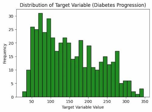
Target Distribution-Geeksforgeeks

This code plots the target variable's distribution as a histogram using the Matplotlib Python module. It designates 30 bins for the histogram, sets the figure size to 6 by 4 inches, and uses green fill instead of black for the edges. The axis labels and caption are added to the plot to give it context. The target variable's frequency of various values, which is connected to the development of diabetes, is plotted as a result.

**Correlation Heatmap or Matrix

A correlation heatmap helps us to understand the relationships between different features in the dataset which shows how features are correlated with each other.

Python3 `

Calculate the correlation matrix

correlation_matrix = np.corrcoef(X, rowvar=False)

Correlation Heatmap

plt.figure(figsize=(8, 4)) sns.heatmap(correlation_matrix, cmap='coolwarm', annot=True, fmt=".2f", xticklabels=diabetes.feature_names, yticklabels=diabetes.feature_names) plt.title('Feature Correlation matrix') plt.show()

**Output:

Confusion Matrix-Geeksforgeeks

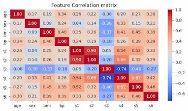
This code computes and displays a dataset's correlation matrix. Using the numpy.corrcoef() function, the correlation matrix is first computed. Next, it uses the seaborn.heatmap() function to produce a heatmap of the correlation matrix. The variables' names are labeled on the x- and y-axes, and the correlation coefficients are noted on the heatmap. The heatmap is finally shown.

Driver function for Bayesian Optimization

Python3 `

Define the objective function for Bayesian Optimization

def catboost_cv(depth, learning_rate, iterations, subsample, l2_leaf_reg): # Convert hyperparameters to the right format depth = int(depth) iterations = int(iterations) l2_leaf_reg = int(l2_leaf_reg) # Initialize the CatBoost model (CatBoostRegressor for regression) model = CatBoostRegressor( depth=depth, learning_rate=learning_rate, iterations=iterations, subsample=subsample, l2_leaf_reg=l2_leaf_reg, verbose=False )

# Perform cross-validation and return the mean R-squared score (for regression)
cross_val_scores = cross_val_score(model, X, y, cv=3, scoring='r2')

return cross_val_scores.mean()

Now we will define a driver function(catboost_cv) before implement Bayesian optimization. Within these function the CatBoost model will be present with all its parameters we are attempting to optimize and cross validation scores will be stored into this function. For validation metric we will use R2-score which is one of the best metric for regression models. The details of parameters are listed below:

**iterations: This parameter is used to specify the number of boosting iterations corresponding to the number of decision trees to be built which controls the overall complexity of the model.
**depth: It defines the depth of each decision tree in the ensemble where a higher depth allows the model to capture more complex relationships present in the data but it may lead to overfitting if set too high.
**learning_rate: The learning rate determines the step size for gradient descent during model training where a smaller learning rate can help to prevent overfitting but may require more iterations to converge.
**subsample: This parameter controls the fraction of data used for each tree during the training process which is essentially a form of stochastic gradient boosting. This helps to reduce overfitting which leads to more robust model.
**l2_leaf_reg: This parameter is responsible for controlling L2 regularization on leaf values which encourages the model to have smaller leaf values and more generalization.
**verbose: These parameter not comes into consideration of any optimization. We can only set it to 'False' to clear the console.

Search space and Bayesian optimization

Now we will define hyperparameter search spaces for each of the hyperparameters of CatBoost model. These will be pass through Bayesian optimization module to achieve optimized values for each hyperparameter.

Python3 `

Define the hyperparameter search space with data types

param_space = { 'depth': (3, 10), # Integer values for depth 'learning_rate': (0.01, 0.3), # Float values for learning rate 'iterations': (100, 1000), # Integer values for iterations 'subsample': (0.5, 1), # Float values for subsample 'l2_leaf_reg': (1, 10) # Integer values for l2_leaf_reg }

Create the BayesianOptimization object and maximize it

bayesian_opt = BayesianOptimization( f=catboost_cv, pbounds=param_space, random_state=42) bayesian_opt.maximize(init_points=5, n_iter=10) results = pd.DataFrame(bayesian_opt.res) results.sort_values(by='target', ascending=False, inplace=True)

**Output:

| iter | target | depth | iterat... | l2_lea... | learni... | subsample |

| 1 | 0.3814 | 5.622 | 955.6 | 7.588 | 0.1836 | 0.578 |
| 2 | 0.4397 | 4.092 | 152.3 | 8.796 | 0.1843 | 0.854 |
| 3 | 0.4 | 3.144 | 972.9 | 8.492 | 0.07158 | 0.5909 |
| 4 | 0.4017 | 4.284 | 373.8 | 5.723 | 0.1353 | 0.6456 |
| 5 | 0.4636 | 7.283 | 225.5 | 3.629 | 0.1162 | 0.728 |
| 6 | 0.4412 | 8.883 | 265.2 | 9.115 | 0.1568 | 0.5336 |
| 7 | 0.4442 | 7.716 | 225.5 | 2.701 | 0.1438 | 0.9897 |
| 8 | 0.4767 | 7.209 | 226.3 | 5.716 | 0.03724 | 0.894 |
| 9 | 0.3897 | 4.119 | 225.4 | 5.436 | 0.2342 | 0.8211 |
| 10 | 0.4042 | 8.471 | 226.9 | 5.505 | 0.2829 | 0.5714 |
| 11 | 0.4672 | 6.903 | 226.5 | 5.264 | 0.07996 | 0.5239 |
| 12 | 0.4142 | 7.961 | 224.7 | 4.326 | 0.2402 | 0.8491 |
| 13 | 0.4266 | 7.069 | 226.3 | 6.76 | 0.2072 | 0.8254 |
| 14 | 0.4151 | 6.948 | 226.3 | 3.913 | 0.1692 | 0.8916 |
| 15 | 0.4183 | 3.935 | 763.5 | 3.712 | 0.06496 | 0.6134 |

The optimal hyperparameters for a CatBoost model are found via Bayesian optimization, which is performed using this code. After defining a hyperparameter search space, it builds an object for Bayesian optimization. It takes five starting points and ten iterations in total to maximize the BayesianOptimization object. The optimization's output is sorted by the target column and saved in a Pandas DataFrame.

Printing best values

Now we will print the best values of hyperparameters and the corresponding R2-score. There is no need to pass these best values of hyperparameters separately to the model. We can directly get the metric value using Bayesian optimization module's build-in feature.

Python3 `

Print the best hyperparameters and their corresponding R2 score

best_hyperparameters = bayesian_opt.max best_hyperparameters['params'] = {param: int(value) if param in [ 'depth', 'iterations', 'l2_leaf_reg'] else value for param, value in best_hyperparameters['params'].items()} print("Best hyperparameters:", best_hyperparameters['params']) print(f"Best R-squared Score: {best_hyperparameters['target']:.4f}")

**Output:

Best hyperparameters: {'depth': 7, 'iterations': 226, 'l2_leaf_reg': 5, 'learning_rate': 0.03724381991311554, 'subsample': 0.8939544712798688}
Best R-squared Score: 0.4767'

This program outputs the optimal hyperparameters following Bayesian optimization together with the related R-squared score. From the Bayesian Optimization object, it first retrieves the optimal hyperparameters. The values for the hyperparameters depth, iterations, or l2_leaf_reg are then transformed as integers. It outputs the R-squared score and optimal hyperparameters to the console at the end.

Visualization of optimization progress

Bayesian Optimization is a multistep calculation where best values of hyperparameters can be achived by testing and fitting the model with different combinations of values and gather the max results as points. The whole can be visualized for better understanding.

Python3 `

param_names = list(param_space.keys())

fig, axes = plt.subplots(2, 3, figsize=(12, 7)) fig.subplots_adjust(hspace=0.4, wspace=0.4) # Adjust spacing

for i, param in enumerate(param_names): if param != 'target': ax = axes[i // 3, i % 3] ax.plot(results['params'].apply(lambda x: x[param]), results['target'], 'bo-', lw=1, markersize=4) ax.set_title(f'Optimization of {param}') ax.set_xlabel(param) ax.set_ylabel('R-squared Score')

    # Mark the best value with a red dot
    best_value = best_hyperparameters['params'][param]
    ax.plot(best_value, best_hyperparameters['target'], 'yo', markersize=6)

Hide any remaining blank subplots

for i in range(len(param_names), 6): fig.delaxes(axes.flatten()[i])

plt.show()

**Output:

catb-Geeksforgeeks

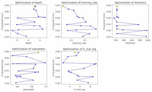
Bayesian optimization progress for each hyperparameter

So, in the plot we can see the optimized values of each hyperparameter with yellow dot and the steps of total optimization process with blue lines.This code creates a plot of the hyperparameter optimization results versus the R-squared score. Initially, a figure with a grid of subplots is created. Next, it plots the optimization results for each hyperparameter after going through the names of each hyperparameter iteratively. Lastly, the figure is displayed and any unfilled subplots are hidden.

Conclusion

Our model's hyperparameters can be optimally tuned with the help of Bayesian optimization, which is a very useful technique. It has allowed us to obtain a reasonably strong R2-Score, indicating that there is room for improvement by investigating different hyperparameter setups. This method has improved our model's performance and shown that it can be used to push the limits of optimization. We may expect to achieve even more optimized outcomes in the future by utilizing Bayesian optimization and investigating a wider range of hyperparameters, which will ultimately improve our model's overall efficacy.