Comparison of Manifold Learning methods in Scikit Learn (original) (raw)
Last Updated : 23 Jul, 2025
**Manifold learning is a **dimensionality reduction techniques which turns complex, high-dimensional data into simpler form while keeping important patterns and features. It works well when the data has curved or non-linear shapes that simple methods like PCA can’t handle. It has several features like:
- Finds and keeps non-linear patterns.
- Makes data easier to see and work with.
- Removes noise and keeps useful info.
- Helps models work better and faster.
Manifold Learning Methods
Scikit-learn provides several manifold learning algorithms. We will use **digits dataset from Scikit-learn which has images of numbers from 0 to 9. Each image is 8×8 pixels giving 64 values leading to many features in data. It consists of various steps:
- Importing required libraries and loading digit images dataset.
- Choosing a manifold learning algorithm.
- Fit the algorithm to the dataset.
- Convert the dataset to a lower-dimensional space.
- Visualizing the converted data.
1. t-SNE (t-distributed Stochastic Neighbor Embedding)
t-SNE is an effective method for visualizing high dimensional data by reducing it to 2D or 3D representations. It is based on the concept of probability distributions and tries to minimize the divergence between the pairwise similarities of data points in high-dimensional space and the similarities in low-dimensional space. This results in a 2D or 3D visualization of the data that retains its inherent structure.
Python `
from sklearn.datasets import load_digits from sklearn.manifold import TSNE import matplotlib.pyplot as plt
digits = load_digits() X = digits.data y = digits.target
tsne = TSNE(n_components=2, random_state=42) X_tsne = tsne.fit_transform(X)
plt.scatter(X_tsne[:, 0], X_tsne[:, 1], c=y) plt.show()
`
**Output:
.png)
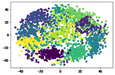
t-SNE
**Interpretation of clusters:
- Points within the same color share similar characteristics.
- Points from different clusters are more distinct from each other.
- Helps to understand the underlying structure of the data.
- Provides a simplified, lower-dimensional view of the data.
2. Isomap (Isometric Mapping)
Isomap is a dimensionality reduction approach based on the idea of geodesic distance. While mapping data points from a higher-dimensional space to a lower-dimensional space. It attempts to retain the geodesic distance between them.
Python `
from sklearn.datasets import load_digits from sklearn.manifold import Isomap import matplotlib.pyplot as plt
digits = load_digits() X = digits.data y = digits.target
isomap = Isomap(n_components=2) X_isomap = isomap.fit_transform(X)
plt.scatter(X_isomap[:, 0], X_isomap[:, 1], c=y) plt.show()
`
**Output:
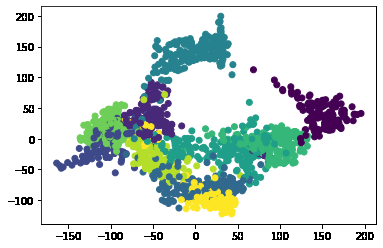
Isomap
**Interpretation of clusters:
- Isomap preserves geodesic distances i.e the shortest paths along the manifold.
- This ensures the overall structure of the data is maintained when mapped into two dimensions.
- It captures the broader relationships within the data.
- Provides a global view of how the data points relate to each other.
3. LLE (Locally Linear Embedding)
Locally Linear Embedding (LLE) is a dimensionality reduction method that seeks to preserve the local structure of the data. It works by attempting to map each point to a lower-dimensional space while maintaining its local neighborhood relationships.
Python `
from sklearn.datasets import load_digits from sklearn.manifold import LocallyLinearEmbedding import matplotlib.pyplot as plt
digits = load_digits() X = digits.data y = digits.target
lle = LocallyLinearEmbedding(n_components=2, random_state=42) X_lle = lle.fit_transform(X)
plt.scatter(X_lle[:, 0], X_lle[:, 1], c=y) plt.show()
`
**Output:
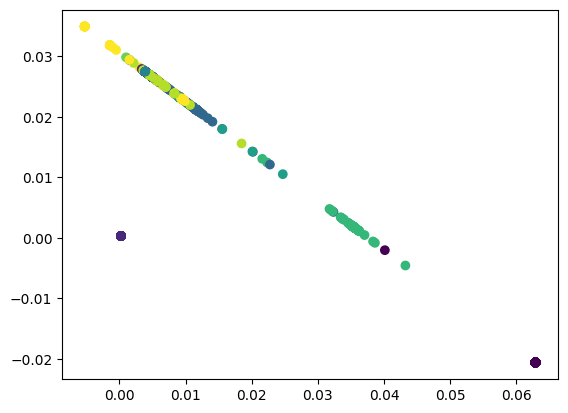
Locally Linear Embedding
**Interpretation of clusters:
- LLE focuses on preserving the local structure of the data.
- Points within the same color are close to each other in high-dimensional space and this proximity is maintained in the 2D projection.
- Data points appear arranged in linear, elongated shapes indicating the intrinsic dimensionality of the data might be lower than expected.
- Tight clusters with different orientations suggest that data points within each cluster are similar to each other.
- The global structure may be somewhat distorted in the 2D projection.
4. MDS (Multi-Dimensional Scaling)
Multi-Dimensional Scaling (MDS) is a dimensionality reduction method that attempts to preserve pairwise distances between points while projecting them into a lower-dimensional space. It is particularly useful when you want to retain the pairwise relationships between data points.
Python `
from sklearn.datasets import load_digits from sklearn.manifold import MDS import matplotlib.pyplot as plt
digits = load_digits() X = digits.data y = digits.target
mds = MDS(n_components=2, random_state=42) X_mds = mds.fit_transform(X)
plt.scatter(X_mds[:, 0], X_mds[:, 1], c=y) plt.show()
`
**Output:
Multi-Dimensional Scaling
**Interpretation of clusters:
- Unlike others it emphasizes the overall distances between points rather than local or geodesic relationships.
- Focuses on maintaining global relationships between data points.
- Aims to preserve the distances between points as much as possible in the 2D space.
Comparison of Methods
Here is the quick comparison of all the methods we learned so far.
| **Method | **Strengths | **Weaknesses | **Ideal Use Cases |
|---|---|---|---|
| **t-SNE | Excellent for visualization of complex, high-dimensional data. Preserves local structures well. | Computationally expensive, can be slow with large datasets, lacks interpretability. | Visualizing high-dimensional data like image or text datasets. |
| **Isomap | Retains geodesic distances, works well with smooth, non-linear manifolds. | Can be slow for large datasets, sensitive to noise. | Data with manifold-like geometry, such as speech data or certain physical phenomena. |
| **LLE | Preserves local neighborhood relationships, good for non-linear data. | Struggles with high curvature or data that doesn’t lie on a smooth manifold. | Non-linear data where local relationships are more important than global structure. |
| **MDS | Preserves pairwise distances, useful for metric data. | Less effective for non-linear data, computationally intensive. | Metric data where preserving distances between points is crucial |
Manifold learning methods like t-SNE, Isomap, LLE and MDS are tools for reducing the dimensionality of high-dimensional data especially when dealing with non-linear structures. Each method has its strengths and weaknesses and choosing the right technique depend on the characteristics of the data and the specific analysis goals.