Image Classification using CNN (original) (raw)

Last Updated : 13 May, 2026

Image classification is a machine learning task where a model assigns labels to images based on their content. CNNs are designed to effectively analyze visual data by learning patterns from images.

Extracts features like edges, shapes, and textures from images.
Learns hierarchical patterns through multiple layers.
Used for tasks like object, scene, and animal classification.

Key Components of CNNs

**Convolutional Layers****:** Filters or kernels that detect features such as edges or textures.
**ReLU Activation****:** Adds non-linearity, helping the model learn complex patterns.
**Pooling Layers****:** Reduce the dimensions of the image making the network more efficient while preserving important features.
**Fully Connected Layers****:** After feature extraction, these layers make the final prediction based on the detected patterns.
**Softmax Output****:** Converts the network’s output into probabilities, showing the likelihood of each class.

CNNs Workflow

**Image preprocessing: Images are resized, normalized, and sometimes augmented to improve model performance and reduce overfitting.
**Feature extraction: CNNs automatically learn hierarchical features, starting from simple edges to complex objects in deeper layers.
**Classification: Fully connected layers use extracted features to assign the image to a predefined class.

Implementation

Let's see the implementation of Image Classification step-by-step:

Step 1: Importing Libraries

Importing Tensorflow and Matplotlib libraries for building, training and visualizing accuracy of the model.

Python `

import tensorflow as tf from tensorflow.keras import layers, models, datasets import matplotlib.pyplot as plt

Step 2: Downloading and Preparing the Dataset

Loading and preprocessing the CIFAR-10 dataset, which contains 60,000 32×32 color images across 10 categories.

**Scaling: Pixel values are normalized from [0, 255] to [0, 1] by dividing by 255.
**One-hot encoding: Converts class labels into binary vectors (e.g., label 2 → [0, 0, 1, 0, 0, 0, 0, 0, 0, 0]). Python `

(x_train, y_train), (x_test, y_test) = datasets.cifar10.load_data()

x_train, x_test = x_train / 255.0, x_test / 255.0

num_classes = 10 y_train = tf.keras.utils.to_categorical(y_train, num_classes) y_test = tf.keras.utils.to_categorical(y_test , num_classes)

**Output:

cnn1

Downloading the Dataset

Step 3: Building the CNN Model

Defining the CNN architecture starting with convolutional and max-pooling layers, followed by flattening and fully connected layers for classification.

**Flatten layer: Converts 2D feature maps into a 1D vector for dense layers.
**Dense layers: Perform final decision making, with softmax used in the output layer to generate class probabilities. Python `

model = models.Sequential([

layers.Conv2D(32, (3,3), activation='relu', padding='same', input_shape=(32,32,3)),
layers.MaxPooling2D(2,2),

layers.Conv2D(64, (3,3), activation='relu', padding='same'),
layers.MaxPooling2D(2,2),

layers.Conv2D(64, (3,3), activation='relu', padding='same'),
layers.Flatten(),

layers.Dense(64, activation='relu'),
layers.Dense(num_classes, activation='softmax')

])

model.summary()

**Output:

cnn2

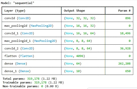
Building the CNN Model

Step 4: Compiling and Training the Model

We compile the model with an optimizer, loss function, and metric, then train it. Adam optimizer is used for adaptive learning rate optimization.

Python `

model.compile(optimizer='adam', loss='categorical_crossentropy', metrics=['accuracy'])

history = model.fit(x_train, y_train, epochs=15, batch_size=64, validation_split=0.2, verbose=2)

**Output:

cnn3

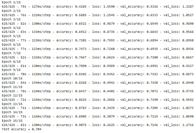
Training the Model

Step 5: Evaluating the Model

We evaluate the trained model on the test dataset to measure its performance on unseen data.

Python `

test_loss, test_acc = model.evaluate(x_test, y_test, verbose=0)

print(f"Test accuracy = {test_acc:.3f}")

Step 6: Making Predictions

We use the trained model to predict the class of unseen test images and compare predicted labels with actual labels.

Python `

predictions = model.predict(x_test)

import numpy as np

Example: predicting first test image

print("Predicted class:", np.argmax(predictions[0])) print("Actual class:", np.argmax(y_test[0]))

**Output:

313/313 ━━━━━━━━━━━━━━━━━━━━ 5s 16ms/step
Predicted class: 3
Actual class: 3

Step7 : Plotting of Accuracy Curves

Using matplotlib to plot and visualize training and validation accuracy during model training.

Python `

plt.plot(history.history['accuracy'], label='train') plt.plot(history.history['val_accuracy'], label='val') plt.legend() plt.title('Accuracy') plt.show()

**Output:

cnn4

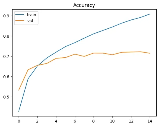
Plotting of Accuracy

Advantages

Automatically learn features from images which reduces manual effort.
Recognize objects regardless of position or orientation.
Reduce computation using pooling layer while retaining key features.
Work well with large datasets and improve with more data.

Challenges

CNNs can overfit on small or complex datasets without proper regularization.
They require high computational power, often needing GPUs or cloud resources.
Performance depends heavily on high-quality, well-labeled data.
Training deep CNNs can be time-consuming with large datasets.