Loan Approval Prediction using Machine Learning (original) (raw)
Last Updated : 23 Jul, 2025
Loans are a major requirement of the modern world. By this alone, banks receive a major portion of the total profit. It is beneficial for students to manage their education and living expenses, and for individuals to purchase various luxuries, such as houses and cars. But when it comes to deciding whether the applicant's profile is relevant to be granted with loan or not. Banks have to look after many aspects.
So, here we will be using machine learning algorithms to ease their work and predict whether the candidate’s profile is relevant or not, using key features like Marital Status, Education, Applicant Income, Credit History, etc.
Loan Approval Prediction using Machine Learning
You can download the used data by visiting this link.
The dataset contains 13 features:
| 1 | Loan | A unique id |
|---|---|---|
| 2 | Gender | Gender of the applicant Male/female |
| 3 | Married | Marital Status of the applicant, values will be Yes/ No |
| 4 | Dependents | It tells whether the applicant has any dependents or not. |
| 5 | Education | It will tell us whether the applicant is Graduated or not. |
| 6 | Self_Employed | This defines that the applicant is self-employed i.e. Yes/ No |
| 7 | ApplicantIncome | Applicant income |
| 8 | CoapplicantIncome | Co-applicant income |
| 9 | LoanAmount | Loan amount (in thousands) |
| 10 | Loan_Amount_Term | Terms of loan (in months) |
| 11 | Credit_History | Credit history of individual's repayment of their debts |
| 12 | Property_Area | Area of property i.e. Rural/Urban/Semi-urban |
| 13 | Loan_Status | Status of Loan Approved or not i.e. Y- Yes, N-No |
Importing Libraries and Dataset
Firstly we have to import libraries:
- Pandas - To load the Dataframe
- Matplotlib - To visualize the data features i.e. barplot
- Seaborn - To see the correlation between features using heatmap Python `
import pandas as pd import numpy as np import matplotlib.pyplot as plt import seaborn as sns
data = pd.read_csv("LoanApprovalPrediction.csv")
`
Once we imported the dataset, let's view it using the below command.
Python `
data.head(5)
`
**Output:
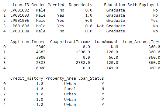
Dataset Loaded
**Data Preprocessing and Visualization
Get the number of columns of object datatype.
Python `
obj = (data.dtypes == 'object') print("Categorical variables:",len(list(obj[obj].index)))
`
**Output :
Categorical variables: 7
As Loan_ID is completely unique and not correlated with any of the other column, So we will drop it using .drop() function.
Python `
Dropping Loan_ID column
data.drop(['Loan_ID'],axis=1,inplace=True)
`
Visualize all the unique values in columns using barplot. This will simply show which value is dominating as per our dataset.
Python `
obj = (data.dtypes == 'object') object_cols = list(obj[obj].index) plt.figure(figsize=(18,36)) index = 1
for col in object_cols: y = data[col].value_counts() plt.subplot(11,4,index) plt.xticks(rotation=90) sns.barplot(x=list(y.index), y=y) index +=1
`
**Output:
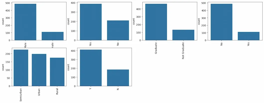
Barplot
As all the categorical values are binary so we can use Label Encoder for all such columns and the values will change into **int datatype.
Python `
Import label encoder
from sklearn import preprocessing
label_encoder object knows how
to understand word labels.
label_encoder = preprocessing.LabelEncoder() obj = (data.dtypes == 'object') for col in list(obj[obj].index): data[col] = label_encoder.fit_transform(data[col])
`
Again check the object datatype columns. Let's find out if there is still any left.
Python `
To find the number of columns with
datatype==object
obj = (data.dtypes == 'object') print("Categorical variables:",len(list(obj[obj].index)))
`
**Output :
Categorical variables: 0
Python `
plt.figure(figsize=(12,6))
sns.heatmap(data.corr(),cmap='BrBG',fmt='.2f', linewidths=2,annot=True)
`
**Output:
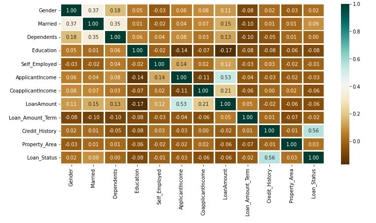
Heatmap
The above heatmap is showing the correlation between Loan Amount and ApplicantIncome. It also shows that Credit_History has a high impact on Loan_Status.
Now we will use Catplot to visualize the plot for the Gender, and Marital Status of the applicant.
Python `
sns.catplot(x="Gender", y="Married", hue="Loan_Status", kind="bar", data=data)
`
**Output:
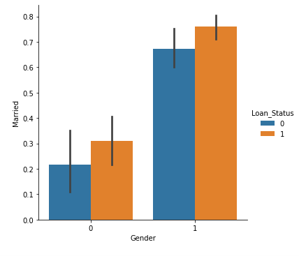
Catplot
Now we will find out if there is any missing values in the dataset using below code.
Python `
for col in data.columns: data[col] = data[col].fillna(data[col].mean())
data.isna().sum()
`
**Output:
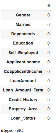
As there is no missing value then we must proceed to model training.
Splitting Dataset
Python `
from sklearn.model_selection import train_test_split
X = data.drop(['Loan_Status'],axis=1) Y = data['Loan_Status'] X.shape,Y.shape
X_train, X_test, Y_train, Y_test = train_test_split(X, Y, test_size=0.4, random_state=1) X_train.shape, X_test.shape, Y_train.shape, Y_test.shape
`
**Output:
((358, 11), (240, 11), (358,), (240,))
Model Training and Evaluation
As this is a classification problem so we will be using these models :
To predict the accuracy we will use the accuracy score function from scikit-learn library.
Python `
from sklearn.neighbors import KNeighborsClassifier from sklearn.ensemble import RandomForestClassifier from sklearn.svm import SVC from sklearn.linear_model import LogisticRegression
from sklearn import metrics
knn = KNeighborsClassifier(n_neighbors=3) rfc = RandomForestClassifier(n_estimators = 7, criterion = 'entropy', random_state =7) svc = SVC() lc = LogisticRegression()
making predictions on the training set
for clf in (rfc, knn, svc,lc): clf.fit(X_train, Y_train) Y_pred = clf.predict(X_train) print("Accuracy score of ", clf.class.name, "=",100*metrics.accuracy_score(Y_train, Y_pred))
`
**Output :
Accuracy score of RandomForestClassifier = 98.04469273743017
Accuracy score of KNeighborsClassifier = 78.49162011173185
Accuracy score of SVC = 68.71508379888269
Accuracy score of LogisticRegression = 80.44692737430168
**Prediction on the test set:
Python `
making predictions on the testing set
for clf in (rfc, knn, svc,lc): clf.fit(X_train, Y_train) Y_pred = clf.predict(X_test) print("Accuracy score of ", clf.class.name,"=", 100*metrics.accuracy_score(Y_test, Y_pred))
`
**Output :
Accuracy score of RandomForestClassifier = 82.5
Accuracy score of KNeighborsClassifier = 63.74999999999999
Accuracy score of SVC = 69.16666666666667
Accuracy score of LogisticRegression = 80.83333333333333
Random Forest Classifier is giving the best accuracy with an accuracy score of 82% for the testing dataset. And to get much better results ensemble learning techniques like **Bagging and **Boosting can also be used.
**You can download the python notebook from here: click here