Linear Discriminant Analysis in Machine Learning (original) (raw)
Last Updated : 13 Sep, 2025
Linear Discriminant Analysis (LDA) also known as Normal Discriminant Analysis is supervised classification problem that helps separate two or more classes by converting higher-dimensional data space into a lower-dimensional space. It is used to identify a linear combination of features that best separates classes within a dataset.
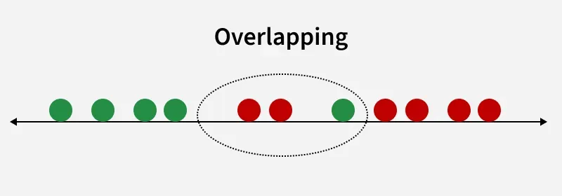
Overlapping
For example we have two classes that need to be separated efficiently. Each class may have multiple features and using a single feature to classify them may result in overlapping. To solve this LDA is used as it uses multiple features to improve classification accuracy. LDA works by some assumptions and we are required to understand them so that we have a better understanding of its working.
**Key Assumptions of LDA
For LDA to perform effectively, certain assumptions are made:
- **Gaussian Distribution: The data in each class should follow a normal bell-shaped distribution.
- **Equal Covariance Matrices: All classes should have the same covariance structure.
- **Linear Separability: The data should be separable using a straight line or plane.
LDA can produce very good results if it meets these assumptions. For example when data points belonging to two classes are plotted, if they are not linearly separable LDA will attempt to find a projection that maximizes class separability.
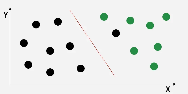
Linearly Separable Dataset
The image shows classes (black and green) that are not linearly separable. LDA finds a new axis (red dashed line) that maximizes the distance between class means while minimizing within-class variance, improving class separation for better classification.
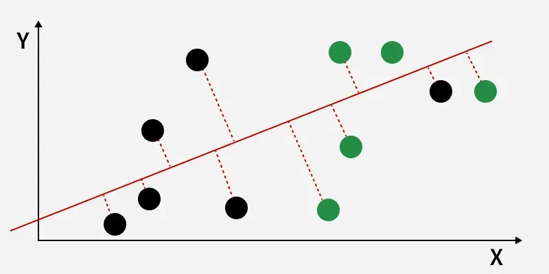
The perpendicular distance between the line and points
The perpendicular distance from the decision boundary to the data points shows how LDA reduces within-class variation and increases class separability. The data points are then projected onto the new axis, as shown in the figure below.
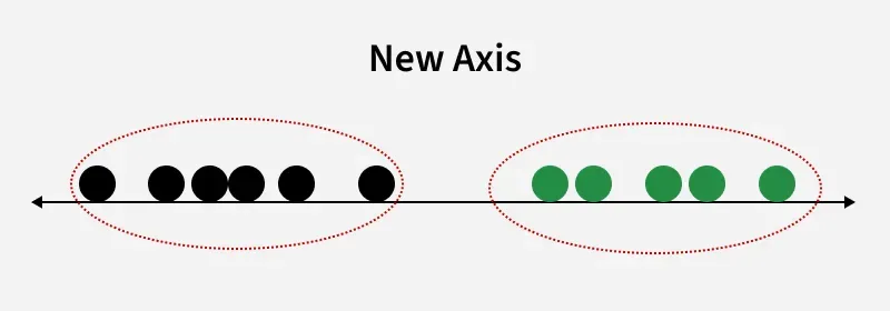
New Axis
This shows how LDA creates a new axis to project the data and separate two classes along a linear path. However, when class distributions share the same mean, LDA cannot find a separating axis and non-linear discriminant analysis is needed.
**How LDA work
LDA works by finding directions in the feature space that best separate the classes. It does this by maximizing the difference between the class means while minimizing the spread within each class.
Let’s assume we have two classes with d-dimensional samples such as x_1, x_2, ... x_n where:
- n_1 samples belong to class c_1
- n_2 samples belong to class c_2.
If x_i represents a data point its projection onto the line represented by the unit vector v is v^T x_i. Let the means of class c_1 and class c_2 before projection be \mu_1 and \mu_2 respectively. After projection the new means are \hat{\mu}_1 = v^T \mu_1 and \hat{\mu}_2 = v^T \mu_2.
Our aim to normalize the difference |\hat{\mu}_1 - \hat{\mu}_2| to maximize the class separation. The scatter for samples of class c_1 is calculated as:
s_1^2 = \sum_{x_i \in c_1} (x_i - \mu_1)^2
Similarly for class c_2:
s_2^2 = \sum_{x_i \in c_2} (x_i - \mu_2)^2
The goal is to maximize the ratio of the between-class scatter to the within-class scatter, which leads us to the following criteria:
J(v) = \frac{|\hat{\mu}_1 - \hat{\mu}_2|}{s_1^2 + s_2^2}
For the best separation we calculate the eigenvector corresponding to the highest eigenvalue of the scatter matrices s_w^{-1} s_b.
**Extensions to LDA
- **Quadratic Discriminant Analysis (QDA): Each class uses its own estimate of variance (or covariance) allowing it to handle more complex relationships.
- **Flexible Discriminant Analysis (FDA): Uses non-linear combinations of inputs such as splines to handle non-linear separability.
- **Regularized Discriminant Analysis (RDA): Introduces regularization into the covariance estimate to prevent overfitting.
Implementation of LDA using Python
We will perform linear discriminant analysis using Scikit-learn library on the Iris dataset.
1. Importing Required Libraries
We import all necessary libraries for data processing, visualization, dimensionality reduction, and modeling
- **NumPy****:** for numerical operations and array manipulations
- **Pandas: for creating and managing structured datasets
- **Matplotlib.pyplot: for plotting and visualizations
- **Scikit-learn: for machine learning tools like dataset loading, preprocessing, dimensionality reduction, and classifiers Python `
import numpy as np import pandas as pd import matplotlib.pyplot as plt from mpl_toolkits.mplot3d import Axes3D from sklearn.datasets import load_iris from sklearn.preprocessing import StandardScaler, LabelEncoder from sklearn.model_selection import train_test_split from sklearn.discriminant_analysis import LinearDiscriminantAnalysis from sklearn.ensemble import RandomForestClassifier from matplotlib.colors import ListedColormap
`
2. Loading the Dataset
We load the Iris dataset and convert it into a Pandas DataFrame. Features X and target labels y are separated
- **pd.DataFrame(columns=..., data=...) creates a DataFrame from raw data
- **iloc[:, 0:4] selects first four columns as features
- **iloc[:, 4] selects the target column Python `
iris = load_iris() dataset = pd.DataFrame(columns=iris.feature_names, data=iris.data) dataset['target'] = iris.target
X = dataset.iloc[:, 0:4].values y = dataset.iloc[:, 4].values
`
3. Data Preprocessing
We scale the features and encode the target labels, then split the dataset into training and testing sets
- **StandardScaler().fit_transform(X) scales features
- **LabelEncoder().fit_transform(y) encodes categorical labels as integers
- **train_test_split(X, y, test_size=0.2, random_state=42) splits data into 80% train and 20% test Python `
sc = StandardScaler() X_scaled = sc.fit_transform(X)
le = LabelEncoder() y_encoded = le.fit_transform(y)
X_train, X_test, y_train, y_test = train_test_split(X_scaled, y_encoded, test_size=0.2, random_state=42)
`
4. Visualizing the Original Iris Dataset in 3D
We create a 3D scatter plot using the first three features to visualize the original data distribution
- Axes3D enables 3D plotting
- **scatter(..., c=y, cmap='rainbow', alpha=0.7, edgecolors='b') colors points by class Python `
fig = plt.figure(figsize=(7,5)) ax = fig.add_subplot(111, projection='3d') ax.scatter(X[:,0], X[:,1], X[:,2], c=y, cmap='rainbow', alpha=0.7, edgecolors='b') ax.set_xlabel(iris.feature_names[0]) ax.set_ylabel(iris.feature_names[1]) ax.set_zlabel(iris.feature_names[2]) ax.set_title('Original Iris Dataset (3D)') plt.show()
`
**Output:
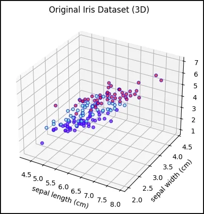
Original Iris Dataset in 3D
5. Random Forest Decision Boundary Without LDA
We train a Random Forest on the original features (first two features only for visualization) and plot the decision boundary
- **RandomForestClassifier(max_depth=2, random_state=0) initialize classifier
- ****.fit(X_train_2D, y_train)** train classifier
- ****.predict()** predict over grid for decision boundary
- **contourf() fills decision regions with colors Python `
X_train_2D = X_train[:, :2]
rf_without_lda = RandomForestClassifier(max_depth=2, random_state=0) rf_without_lda.fit(X_train_2D, y_train)
x_min, x_max = X_train_2D[:,0].min() - 1, X_train_2D[:,0].max() + 1 y_min, y_max = X_train_2D[:,1].min() - 1, X_train_2D[:,1].max() + 1 xx, yy = np.meshgrid(np.arange(x_min, x_max, 0.02), np.arange(y_min, y_max, 0.02))
Z = rf_without_lda.predict(np.c_[xx.ravel(), yy.ravel()]) Z = Z.reshape(xx.shape) cmap_light = ListedColormap(['#FFAAAA', '#AAFFAA', '#AAAAFF'])
plt.figure(figsize=(7,5)) plt.contourf(xx, yy, Z, alpha=0.3, cmap=cmap_light) plt.scatter(X_train_2D[:,0], X_train_2D[:,1], c=y_train, cmap='rainbow', edgecolors='b') plt.xlabel(iris.feature_names[0]) plt.ylabel(iris.feature_names[1]) plt.title('Random Forest Decision Boundary Without LDA') plt.show()
`
**Output:
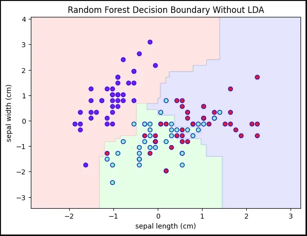
Decision Boundary Without LDA
6. Applying LDA
We reduce the feature space to 2 components to maximize class separability
- **LinearDiscriminantAnalysis(n_components=2) reduces features to 2 components
- ****.fit_transform(X_train, y_train)** fit LDA on training data and transform it
- ****.transform(X_test)** project test data onto same LDA components Python `
lda = LinearDiscriminantAnalysis(n_components=2) X_train_lda = lda.fit_transform(X_train, y_train) X_test_lda = lda.transform(X_test)
`
7. Random Forest Decision Boundary With LDA
We train a Random Forest on LDA-transformed features and plot its decision boundary
- **RandomForestClassifier(max_depth=2, random_state=0) initialize classifier
- ****.fit(X_train_lda, y_train)** train classifier
- ****.predict()** predict over grid for decision boundary
- **contourf() fills decision regions with colors Python `
rf_with_lda = RandomForestClassifier(max_depth=2, random_state=0) rf_with_lda.fit(X_train_lda, y_train)
x_min, x_max = X_train_lda[:,0].min() - 1, X_train_lda[:,0].max() + 1 y_min, y_max = X_train_lda[:,1].min() - 1, X_train_lda[:,1].max() + 1 xx, yy = np.meshgrid(np.arange(x_min, x_max, 0.02), np.arange(y_min, y_max, 0.02))
Z = rf_with_lda.predict(np.c_[xx.ravel(), yy.ravel()]) Z = Z.reshape(xx.shape)
plt.figure(figsize=(7,5)) plt.contourf(xx, yy, Z, alpha=0.3, cmap=cmap_light) plt.scatter(X_train_lda[:,0], X_train_lda[:,1], c=y_train, cmap='rainbow', edgecolors='b') plt.xlabel('LDA Component 1') plt.ylabel('LDA Component 2') plt.title('Random Forest Decision Boundary With LDA') plt.show()
`
**Output:
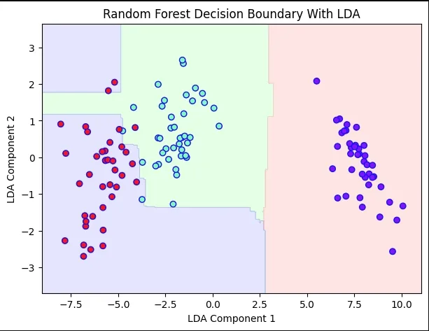
Decision Boundary With LDA
**Advantages of LDA
- Simple and computationally efficient.
- Works well even when the number of features is much larger than the number of training samples.
- Can handle multicollinearity.
**Disadvantages of LDA
- Assumes Gaussian distribution of data which may not always be the case.
- Assumes equal covariance matrices for different classes which may not hold in all datasets.
- Assumes linear separability which is not always true.
- May not always perform well in high-dimensional feature spaces.
**Applications of LDA
- **Face Recognition: It is used to reduce the high-dimensional feature space of pixel values in face recognition applications helping to identify faces more efficiently.
- **Medical Diagnosis: It classifies disease severity in mild, moderate or severe based on patient parameters helping in decision-making for treatment.
- **Customer Identification: It can help identify customer segments most likely to purchase a specific product based on survey data.