Multidimensional image processing using Scipy in Python (original) (raw)
Last Updated : 23 Jul, 2025
SciPy is a Python library used for scientific and technical computing. It is built on top of NumPy, a library for efficient numerical computing, and provides many functions for working with arrays, numerical optimization, signal processing, and other common tasks in scientific computing.
Image processing is the field of computer science that deals with the manipulation, analysis, and interpretation of images. In image processing, a multidimensional image is an image that has more than two dimensions. This can include images with multiple color channels (e.g., red, green, and blue channels in a color image), images with multiple time points (e.g., a video), and images with multiple spatial dimensions (e.g., a 3D medical imaging scan).
SciPy provides several functions for processing multidimensional images, including functions for reading and writing images, image filtering, image warping, and image segmentation. The 'scipy.ndimage' is a module in the SciPy library that provides functions for multidimensional image processing. It is built on top of NumPy, a library for efficient numerical computing, and provides many functions for working with arrays, including functions for image processing.
Since there are a lot of operations possible, the article covers some of the basic operations
- Image filtering: We can use the scipy.ndimage.filters module to apply various types of image filters, such as median filters, Gaussian filters, and Sobel filters.
- Image interpolation: We can use the scipy.ndimage.interpolation module to warp images using various interpolation methods, such as nearest-neighbor, linear, and cubic.
- Image segmentation: We can use the scipy.ndimage.measurements module to perform image segmentation tasks, such as finding connected components and labeling objects in an image.
- Image manipulation: We can use the scipy.ndimage.morphology module to perform image manipulation tasks, such as erosion, dilation, and opening and closing.
Image Filtering with SciPy
In image processing, filters are mathematical operations that are applied to an image to modify its appearance or extract specific features. Filters can be used for tasks such as smoothing, sharpening, enhancing edges, removing noise, and more. Many types of filters can be used in image processing, including linear filters, non-linear filters, and morphological filters. Linear filters apply a linear combination of the input image pixels to produce the output image, while non-linear filters apply a non-linear function to the input image pixels. Morphological filters are a type of non-linear filter that is based on the shape or structure of the image pixels.
The scipy.ndimage module in particular provides several filter functions for tasks such as smoothing, sharpening, and edge detection.
Here are some examples of filter functions that are provided by scipy.ndimage:
- Median filter: We can use the scipy.ndimage.filters.median_filter function to apply a median filter to an image, which can be used to remove noise from the image.
- Gaussian filter: We can use the scipy.ndimage.filters.gaussian_filter function to apply a Gaussian filter to an image, which can be used to smooth the image or reduce noise.
- Sobel filter: We can use the scipy.ndimage.filters.sobel function to apply a Sobel filter to an image, which is a type of edge detection filter that enhances edges in the image.
- Laplacian filter: We can use the scipy.ndimage.filters.laplace function to apply a Laplacian filter to an image, which is a second-order derivative filter that can be used to detect edges and corners in the picture.
- Prewitt filter: The Prewitt filter is a type of edge detection filter that is similar to the Sobel filter. It calculates the gradient of the image intensity and enhances edges in the image by identifying areas of rapid intensity change. We can use the scipy.ndimage.filters.prewitt function to apply a Prewitt filter to an image.
| Filter Function | Syntax | Parameters |
|---|---|---|
| Median Filter | scipy.ndimage.median_filter(input, size=None, footprint=None, output=None, mode='reflect', cval=0.0, origin=0) | The size parameter specifies the size of the filter, which can be a scalar or a tuple of integers. For example, a size of 3 will apply a 3x3 median filter, while a size of (3, 5) will apply a 3x5 median filter. The footprint parameter allows you to specify the shape of the filter, which can be a Boolean array or a sequence of indices. The mode parameter specifies how the edges of the image are handled, with options such as 'reflect', 'wrap', and 'constant'. |
| Gaussian Filter | scipy.ndimage.gaussian_filter(input, sigma, order=0, output=None, mode='reflect', cval=0.0, truncate=4.0) | The sigma parameter specifies the standard deviation of the Gaussian function, which determines the amount of smoothing applied to the image. The order parameter allows you to specify the order of the derivative to be applied, with options such as 0 for smoothing, 1 for first derivative, and 2 for the second derivative. |
| Sobel Filter | scipy.ndimage.sobel(input, axis=- 1, output=None, mode='reflect', cval=0.0) | The axis parameter allows you to specify the direction of the filter, with 0 for horizontal and 1 for vertical. |
| Laplace Filter | scipy.ndimage.laplace(input, output=None, mode='reflect', cval=0.0) | The size parameter allows you to specify the size of the filter, which can be a scalar or a tuple of integers. For example, a size of 3 will apply a 3x3 Laplacian filter, while a size of (3, 5) will apply a 3x5 Laplacian filter. |
| Prewitt Filter | scipy.ndimage.prewitt(input, axis=- 1, output=None, mode='reflect', cval=0.0) | With the axis set to 0 for horizontal and 1 for vertical, you can choose the filter's direction. With options like 0 for smoothing, 1 for the first derivative, and 2 for the second derivative, the order parameter enables you to choose the order of the derivative. The mode parameter, which has possibilities including "reflect," "wrap," and "constant," describes how the image's edges are handled. |
Here is a code snippet showing the implementation of all the filters.
Python3 `
Import the necessary libraries
import scipy.ndimage from scipy import misc import matplotlib.pyplot as plt
reads a raccoon face
image = misc.face() #image = plt.imread('Ganesh.jpg')
Apply a Gaussian filter to the image
gaussian_filtered_image = scipy.ndimage.filters.gaussian_filter(image, sigma=3)
Apply Median Filter
median_filtered_image = scipy.ndimage.filters.median_filter(image, size=3)
Apply Sobel Filter
sobel_filtered_image = scipy.ndimage.filters.sobel(image)
Apply Laplace Filter
laplace_filtered_image = scipy.ndimage.filters.laplace(image)
Apply Prewitt Filter
prewitt_filtered_image = scipy.ndimage.filters.prewitt(image)
Initialise the subplot function using number of rows and columns
figure, axis = plt.subplots(3, 2, figsize=(8, 8))
original image
axis[0, 0].imshow(image) axis[0, 0].set_title("Original Image") axis[0, 0].axis('off')
gaussian filter
axis[0, 1].imshow(gaussian_filtered_image) axis[0, 1].set_title("Gaussian Filtered Image") axis[0, 1].axis('off')
median filter
axis[1, 0].imshow(median_filtered_image) axis[1, 0].set_title("Median Filtered Image") axis[1, 0].axis('off')
sobel filter
axis[1, 1].imshow(sobel_filtered_image) axis[1, 1].set_title("Sobel Filtered Image") axis[1, 1].axis('off')
laplace filter
axis[2, 1].imshow(laplace_filtered_image) axis[2, 1].set_title("Laplace Filtered Image") axis[2, 1].axis('off')
prewitt filter
axis[2, 0].imshow(prewitt_filtered_image) axis[2, 0].set_title("Prewitt Filtered Image") axis[2, 0].axis('off')
plt.show()
`
Outputs:
.png)
Image Filtering with SciPy
Image Interpolation with scipy
Image interpolation is the process of estimating the values of pixels in an image based on the values of surrounding pixels. Image interpolation is often used to resize images or to correct distortions in images.
There are several different methods of interpolation that can be used for image processing, including nearest neighbor interpolation, bilinear interpolation, and bicubic interpolation. The choice of interpolation method can affect the quality and smoothness of the resulting image, as well as the computational complexity of the interpolation process.
Here are different types of interpolation transformations provided in the scipy.ndimage.
- **Affine transformation:**- An affine transformation is a linear transformation that preserves lines and parallelism. It is a type of transformation that can be used to rotate, scale, translate, or skew an image.
- Zoom:- The zoom function allows one to zoom in or out on an image by interpolating the values of the pixels. This can be useful for tasks such as image resizing or image analysis, where one may want to change the size of an image or examine the image at different scales.
- Shift:- It allows to shift of an image by a specified amount. This can be useful for tasks such as image alignment or image analysis, where one may want to compare slightly offset images.
- Rotate:- It allows the rotation of an image by a specific amount. This can be useful for tasks such as image alignment or image analysis, where one may want to compare slightly offset images.
- Spline filter:- A spline filter is a type of smoothing filter that uses a spline function to fit a curve to the values of the pixels in the image. This can be useful for tasks such as image denoising or image smoothing, where you may want to reduce noise or smooth out rough edges in the image.
| Interpolation Functions | Syntax | Parameters |
|---|---|---|
| Affine transformation | scipy.ndimage.affine_transform(input, matrix, offset=0.0, output_shape=None, output=None, order=3, mode='constant', cval=0.0, prefilter=True) | output_shape: This parameter allows you to specify the size and shape of the output image. It should be a tuple of integers. output_center: This parameter allows you to specify the center of the output image. It should be a tuple of floats. mode: This parameter specifies how the edges of the image are handled, with options such as 'reflect', 'wrap', and 'constant'. |
| Zoom | scipy.ndimage.zoom(input, zoom, output=None, order=3, mode='constant', cval=0.0, prefilter=True, *, grid_mode=False) | The zoom parameter specifies the zoom factor, which can be a scalar or a tuple of floats. For example, a zoom factor of 2 will double the size of the image, while a zoom factor of (2, 1) will double the width and leave the height unchanged |
| Shift | scipy.ndimage.shift(input, shift, output=None, order=3, mode='constant', cval=0.0, prefilter=True) | The shift parameter specifies the shift amount as a tuple of floats, with the first element specifying the shift in the x direction and the second element specifying the shift in the y direction. |
| Rotate | scipy.ndimage.rotate(input, angle, axes=(1, 0), reshape=True, output=None, order=3, mode='constant', cval=0.0, prefilter=True) | reshape: This parameter specifies whether the output image should be resized to fit the entire rotated image. By default, the output image has the same size as the input image. |
| spline filter | scipy.ndimage.spline_filter(input, order=3, output=<class 'numpy.float64'>, mode='mirror') | order: This parameter allows you to specify the interpolation method to be used, with options such as 0 for nearest neighbor interpolation, 1 for bilinear interpolation, and 3 for bicubic interpolation. |
Here is a code snippet showing the implementation of all the Interpolation methods.
Python3 `
Import the necessary libraries
import scipy.ndimage from scipy import misc import numpy as np import matplotlib.pyplot as plt
reads a image
image = misc.ascent()
apply Affline transformation
w, h = image.shape
Rotate the image by 30° counter-clockwise.
theta = np.pi/6
first shift/center the image, apply rotation,and then apply inverse shift
mat_rotate = np.array( [[1, 0, w/2], [0, 1, h/2], [0, 0, 1]]) @ np.array( [[np.cos(theta), np.sin(theta), 0], [np.sin(theta), -np.cos(theta), 0], [0, 0, 1]]) @ np.array( [[1, 0, -w/2], [0, 1, -h/2], [0, 0, 1]])
affine transformation
affline_transformed_image = scipy.ndimage.affine_transform(image, mat_rotate)
Resize the image using bilinear interpolation with zoom
resized_image = scipy.ndimage.interpolation.zoom(image, zoom=2, order=1)
Shift the image by (10, 20) pixels
shifted_image = scipy.ndimage.interpolation.shift(image, shift=(10, 20))
Rotate the image by 45 degrees
rotated_image = scipy.ndimage.interpolation.rotate(image, angle=45)
Apply the spline filter to the image
filtered_image = scipy.ndimage.interpolation.spline_filter(image)
Initialise the subplot function using number of rows and columns
figure, axis = plt.subplots(3, 2, figsize=(8, 8))
original image
axis[0, 0].imshow(image) axis[0, 0].set_title("Original Image") axis[0, 0].axis('off')
affline transformation filter
axis[0, 1].imshow(affline_transformed_image) axis[0, 1].set_title("affline_transformed_image") axis[0, 1].axis('off')
zoom filter
axis[1, 0].imshow(resized_image) axis[1, 0].set_title("resized_image") axis[1, 0].axis('off')
rotate filter
axis[1, 1].imshow(rotated_image) axis[1, 1].set_title("rotated_image") axis[1, 1].axis('off')
shift filter
axis[2, 1].imshow(shifted_image) axis[2, 1].set_title("shifted_image") axis[2, 1].axis('off')
spline filter
axis[2, 0].imshow(filtered_image) axis[2, 0].set_title("spline_filter_image") axis[2, 0].axis('off')
plt.show()
`
Output:
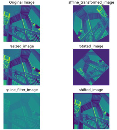
Image Interpolation with scipy
Image Segmentation using Scipy
Image segmentation is the process of dividing an image into different regions or segments based on specific criteria. It is a common technique used in image processing and computer vision applications to identify and extract objects or regions of interest in an image.
The scipy.ndimage.measurements module of the scipy library provides a number of functions that can be used for image segmentation. Here are a few examples:
- scipy.ndimage.measurements.label: This function allows you to label connected components in an image. It is often used as a preprocessing step for segmenting objects in an image.
- scipy.ndimage.measurements.mean: This function allows you to calculate the mean of the values of an image or array.
- scipy.ndimage.measurements.variance: This function allows you to calculate the variance of the values of an image or array.
- scipy.ndimage.measurements.standard_deviation: This function allows you to calculate the standard deviation of the values of an image or array.
- scipy.ndimage.measurements.center_of_mass: This function allows you to calculate the center of mass of an image or region of an image. It can be used to identify the locations of objects in an image.
Here is a code snippet showing the implementation of the label measurement function.
Python3 `
#Import the necessary libraries import scipy.ndimage import numpy as np import matplotlib.pyplot as plt from scipy import misc
Read the image
image = misc.face()
Convert the image to grayscale
image = np.mean(image, axis=2)
Threshold the image to create a binary image
threshold = 128 binary_image = image > threshold
Label the connected components in the binary image
labels, num_labels = scipy.ndimage.label(binary_image)
plotting image
f = plt.figure()
original image
f.add_subplot(1,2, 1) plt.imshow(image) plt.title('Original image') plt.axis("off")
labeled Image
f.add_subplot(1,2, 2) plt.imshow(labels) plt.title("Labeled Image") plt.axis("off")
plt.show(block=True)
`
Output:
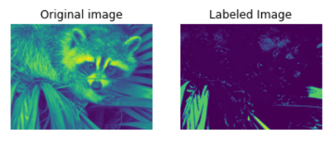
Image Segmentation using Scipy
Implementation of several other measurement functionalities provided by the ndimage library are shown in the code below
Python3 `
#Import the necessary libraries import scipy.ndimage import numpy as np import matplotlib.pyplot as plt from scipy import misc
Read the image
image = misc.face()
Convert the image to grayscale
image = np.mean(image, axis=2)
Threshold the image to create a binary image
threshold = 128 binary_image = image > threshold
extrema
min_value, max_value, min_loc, max_loc = scipy.ndimage.extrema(image)
mean value
mean = scipy.ndimage.mean(image)
calculate center of mass
center_of_mass = scipy.ndimage.center_of_mass(image)
standard deviation
standard_deviation= scipy.ndimage.standard_deviation(image)
variance
variance = scipy.ndimage.variance(image)
print("Minimum pixel value in the image is {} on the location {}".format(min_value, min_loc)) print("Maximum pixel value in the image is {} on the location {}".format(max_value,max_loc)) print("Mean:- {} \nCenter of Mass:- {} \nStandard Deviation:- {} \nVariance:- {}".format( mean, center_of_mass, standard_deviation, variance))
`
Output:-
Minimum pixel value in the image is 0.3333333333333333 on the location (567, 258) Maximum pixel value in the image is 254.0 on the location (245, 568) Mean:- 110.16274388631183 Center of Mass:- (356.6752247435916, 469.240201083681) Standard Deviation:- 54.975712030326186 Variance:- 3022.3289132413515
Image Manipulation with Scipy
The scipy.ndimage.morphology module of the scipy library provides a number of functions for performing morphological operations on images. Morphological operations are a set of image-processing techniques that involve the use of shapes or structuring elements to process images. These operations are often used for tasks such as image enhancement, noise reduction, and object extraction.
Here are a few examples of morphological operations that are available in scipy.ndimage.morphology:
- scipy.ndimage.morphology.binary_erosion: This function allows you to apply binary erosion to an image, which can be used to thin or remove small features from the image.
- scipy.ndimage.morphology.binary_dilation: This function allows you to apply binary dilation to an image, which can be used to thicken or add small features to the image.
- scipy.ndimage.morphology.binary_closing: This function allows you to apply morphological closing to an image, which can be used to fill small holes or remove small objects from the image.
- scipy.ndimage.morphology.binary_opening: This function allows you to apply morphological opening to an image, which can be used to remove small objects or fill small holes in the image.
The code snippet shows the working of all the above-mentioned functions
Python3 `
#Import the necessary libraries import scipy.ndimage import numpy as np import matplotlib.pyplot as plt from scipy import misc
Read the image
image = misc.face()
Convert the image to grayscale
image = np.mean(image, axis=2)
Threshold the image to create a binary image
threshold = 128 binary_image = image > threshold
Create a structuring element for the closing operation
structuring_element = np.ones((10, 10), dtype=np.bool_)
Apply morphological closing to the binary image
closed_image = scipy.ndimage.morphology.binary_closing(binary_image, structure=structuring_element)
Apply morphological opening to the binary image
opened_image = scipy.ndimage.morphology.binary_opening(binary_image, structure=structuring_element)
Apply morphological binary erosion to the binary image
binary_erosion_image = scipy.ndimage.morphology.binary_erosion(binary_image, structure=structuring_element)
Apply morphological binary dilation to the binary image
binary_dilation_image = scipy.ndimage.morphology.binary_dilation(binary_image, structure=structuring_element)
Apply morphological binary fill holes to the binary image
binary_fill_holes = scipy.ndimage.binary_fill_holes(binary_image, structure=structuring_element)
Initialise the subplot function using number of rows and columns
figure, axis = plt.subplots(3, 2, figsize = (8,8))
original image
axis[0, 0].imshow(image) axis[0, 0].set_title("Original Image") axis[0, 0].axis('off')
closed_image
axis[0, 1].imshow(closed_image) axis[0, 1].set_title("Binary closed image") axis[0, 1].axis('off')
Opened Image
axis[1, 0].imshow(opened_image) axis[1, 0].set_title("Binary Opened Image") axis[1, 0].axis('off')
Erosion image
axis[1, 1].imshow(binary_erosion_image) axis[1, 1].set_title("Erosion image") axis[1, 1].axis('off')
Dilation image
axis[2, 1].imshow(binary_dilation_image) axis[2, 1].set_title("Dilation image") axis[2, 1].axis('off')
Fill holes
axis[2, 0].imshow(binary_fill_holes ) axis[2, 0].set_title("Fill holes") axis[2, 0].axis('off')
plt.show()
`
Output:
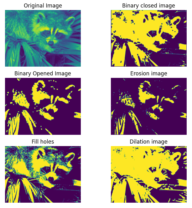
Image Manipulation with Scipy