Music Genre Classifier using Machine Learning (original) (raw)

Last Updated : 23 Jul, 2025

Music is the art of arranging sound and noise together to create harmony, melody, rhythm, and expressive content. It is organized so that humans and sometimes other living organisms can express their current emotions with it.

We all have our own playlist, which we listen to while traveling, studying, dancing, etc.

In short, every emotion has a different genre. So here today, we will study how can we implement the task of genre classification using Machine Learning in Python.

Before starting the code, download the data from this link.

Let's start with the code.

Import Libraries and Dataset

Firstly we need to import Libraries :

• Pandas: To import files/datasets.
• Matplotlib: To visualize the data frame.
• Numpy: To perform operations like scaling and correlation.
• Seaborn: To visualize the data frame.
• Librosa: To visualize the audio data. Install this library by "pip install librosa" command. Python3 `

import numpy as np import pandas as pd import matplotlib.pyplot as plt import seaborn as sns import librosa.display

`

Now to import the data file run the below command.

Python3 `

music_data = pd.read_csv('file.csv') music_data.head(5)

`

Output :

Exploratory Data Analysis

Let's find out the count of each music label.

Python3 `

music_data['label'].value_counts()

`

Output:

blues 100 classical 100 country 100 disco 100 hiphop 100 jazz 100 metal 100 pop 100 reggae 100 rock 100

We can also analysis the sound waves of the audio using the Librosa library.

Let's visualize few of them with the below code.

Python3 `

path = 'genres_original/blues/blues.00000.wav' plt.figure(figsize=(14, 5)) x, sr = librosa.load(path) librosa.display.waveplot(x, sr=sr) id.Audio(path)

print("Blue")

`

Output :

Blue

Python3 `

path = 'genres_original/metal/metal.00000.wav' plt.figure(figsize=(14, 5)) x, sr = librosa.load(path) librosa.display.waveplot(x, sr=sr,color='orange') id.Audio(path)

print("Metal")

`

Output :

Metal

Python3 `

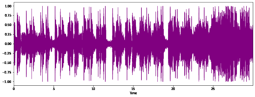
path = 'genres_original/pop/pop.00000.wav' plt.figure(figsize=(14, 5)) x, sr = librosa.load(path) librosa.display.waveplot(x, sr=sr,color='purple') id.Audio(path)

print("Pop")

`

Output :

Pop

Python3 `

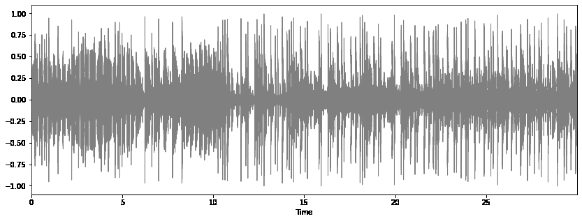
path = 'genres_original/hiphop/hiphop.00000.wav' plt.figure(figsize=(14, 5)) x, sr = librosa.load(path) librosa.display.waveplot(x, sr=sr,color='grey') id.Audio(path)

print("HipHop")

`

Output :

HipHop

Python3 `

import numpy as np import seaborn as sns

Computing the Correlation Matrix

spike_cols = [col for col in data.columns if 'mean' in col]

Set up the matplotlib figure

f, ax = plt.subplots(figsize=(16, 11));

Draw the heatmap with the mask and correct aspect ratio

sns.heatmap(data[spike_cols].corr(), cmap='YlGn')

plt.title('Heatmap for MEAN variables', fontsize = 20) plt.xticks(fontsize = 10) plt.yticks(fontsize = 10);

`

Output :

Data Preprocessing

Initially, we need to use LabelEncoder() to convert the labels into integer.

Python3 `

from sklearn import preprocessing label_encoder = preprocessing.LabelEncoder() music_data['label'] = label_encoder.fit_transform(music_data['label'])

`

As filename column is not a relevant, so we can drop it.

Python3 `

X = music_data.drop(['label','filename'],axis=1) y = music_data['label']

`

Now the data needs to be scaled, to make the model more stable and train fast.

Python3 `

cols = X.columns minmax = preprocessing.MinMaxScaler() np_scaled = minmax.fit_transform(X)

new data frame with the new scaled data.

X = pd.DataFrame(np_scaled, columns = cols)

`

Model Training

Initially, split the model using train_test_split module.

Python3 `

from sklearn.model_selection import train_test_split

X_train, X_test, y_train, y_test = train_test_split(X, y, test_size=0.3, random_state=111) X_train.shape, X_test.shape, y_train.shape, y_test.shape

`

We will be testing our datasets on below models :

• K-Neighbors Classifier : KNeighborsClassifier looks for topmost n_neighbors using different distance methods like Euclidean distance.
• Decision Tree Classifier : In Decision tree each node is trained by splitting the data is continuously according to a certain parameter.
• Random Forest : Random Forest Classifier fits a number of decision tree classifiers on many sub-samples of the dataset and then use the average to improve the results.
• Logistics Regression : Logistic Regression is a regression model that predicts the probability of a given data belongs to the particular category or not.
• Cat Boost : CatBoost implements decision trees and restricts the features split per level to one, which help in decreasing prediction time. It also handles categorical features effectively.
• Gradient Boost : In Gradient Boost an decision trees are implemented in a sequential manner which enhance the performance. Python3 `

from sklearn.metrics import accuracy_score from sklearn.neighbors import KNeighborsClassifier from sklearn.tree import DecisionTreeClassifier from sklearn.ensemble import RandomForestClassifier from sklearn.linear_model import LogisticRegression import catboost as cb from xgboost import XGBClassifier

rf = RandomForestClassifier(n_estimators=1000, max_depth=10, random_state=0) cbc = cb.CatBoostClassifier(verbose=0, eval_metric='Accuracy', loss_function='MultiClass') xgb = XGBClassifier(n_estimators=1000, learning_rate=0.05)

for clf in (rf, cbc, xgb): clf.fit(X_train, y_train) preds = clf.predict(X_test) print(clf.class.name,accuracy_score(y_test, preds))

`

Output :

RandomForestClassifier 0.78 CatBoostClassifier 0.8333333333333334 XGBClassifier 0.7933333333333333

Neural Network

Let's evaluate the dataset with the simple Neural network.

Python3 `

import tensorflow.keras as keras from tensorflow.keras import Sequential from tensorflow.keras.layers import *

model = Sequential()

model.add(Flatten(input_shape=(58,))) model.add(Dense(256, activation='relu')) model.add(BatchNormalization()) model.add(Dense(128, activation='relu')) model.add(Dropout(0.3)) model.add(Dense(10, activation='softmax')) model.summary()

`

Output :

Compiling and fitting the model

Python3 `

compile the model

adam = keras.optimizers.Adam(lr=1e-4) model.compile(optimizer=adam, loss="sparse_categorical_crossentropy", metrics=["accuracy"])

hist = model.fit(X_train, y_train, validation_data = (X_test,y_test), epochs = 100, batch_size = 32)

`

100 epochs will take some time.

Once done, then we can do evaluation.

Evaluation

Let's check the test accuracy by below code.

Python3 `

test_error, test_accuracy = model.evaluate(X_test, y_test, verbose=1) print(f"Test accuracy: {test_accuracy}")

`

Output :

Test accuracy: 0.7566666603088379

Now we can evaluate the accuracy using line-plots.

Python3 `

fig, axs = plt.subplots(2,figsize=(10,10))

accuracy

axs[0].plot(hist.history["accuracy"], label="train") axs[0].plot(hist.history["val_accuracy"], label="test")
axs[0].set_ylabel("Accuracy") axs[0].legend() axs[0].set_title("Accuracy")

Error

axs[1].plot(hist.history["loss"], label="train") axs[1].plot(hist.history["val_loss"], label="test")
axs[1].set_ylabel("Error") axs[1].legend() axs[1].set_title("Error")

plt.show()

`

Output :

Conclusion

Ensemble Learning and Neural nets has been proven the best way for classification of the genre with the accuracy of more than 80%