Optimization Algorithms in Machine Learning (original) (raw)

Last Updated : 9 May, 2026

Machine learning models learn by minimizing a loss function that measures the difference between predicted and actual values. Optimization algorithms are used to update model parameters so that this loss is reduced and the model learns better from data. Their main roles in training include:

• Adjust model parameters to minimize the loss function.
• Help models improve predictions through repeated updates.
• Move the model toward an optimal solution during training.

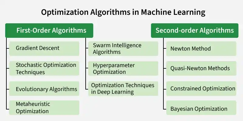
Optimization Algorithms

First Order Algorithms

First order optimization algorithms use the first derivative (gradient) of the loss function to update model parameters and move toward an optimal solution. They are widely used in machine learning because they are computationally efficient and scale well to large datasets.

1. Gradient Descent

Gradient Descent is a first order optimization algorithm used to minimize a loss function by updating model parameters step by step in the direction that reduces the error. It is widely used in machine learning and deep learning to train models efficiently.

• **Compute gradient: Calculate the derivative of the loss function at the current parameters.
• **Update parameters: Move parameters in the opposite direction of the gradient using a learning rate.
• **Repeat process: Continue updating parameters for multiple iterations.
• **Reach minimum: Parameters gradually move toward values that minimize the loss.

**Implementation

• **Defines the function and its gradient: Specifies the function and how its slope is calculated.
• **Applies Gradient Descent: Starts from an initial value and updates it repeatedly using the learning rate.
• **Checks convergence: Stops when the change in the value becomes very small.
• **Visualizes the optimization: Plots the function and shows how Gradient Descent moves toward the minimum point. Python `

import numpy as np import matplotlib.pyplot as plt def function(x): return x**2 def gradient(x): return 2 * x def gradient_descent(start, learning_rate=0.1, n_iter=50, tolerance=1e-6): x = start history = [x]

for i in range(n_iter):
    grad = gradient(x)
    new_x = x - learning_rate * grad
    
    if abs(new_x - x) < tolerance:
        print(f"Converged at iteration {i+1}")
        break
    
    x = new_x
    history.append(x)

return x, history

start = 5.0
learning_rate = 0.1
n_iter = 50
tolerance = 1e-6
result, history = gradient_descent(start, learning_rate, n_iter, tolerance) print("Final optimized value of x:", result) print("Minimum value of f(x):", function(result)) x_vals = np.linspace(-6, 6, 400) y_vals = function(x_vals) plt.figure() plt.plot(x_vals, y_vals) plt.scatter(history, [function(x) for x in history]) plt.title("Gradient Descent Optimization") plt.xlabel("x") plt.ylabel("f(x) = x^2") plt.show()

`

**Output:

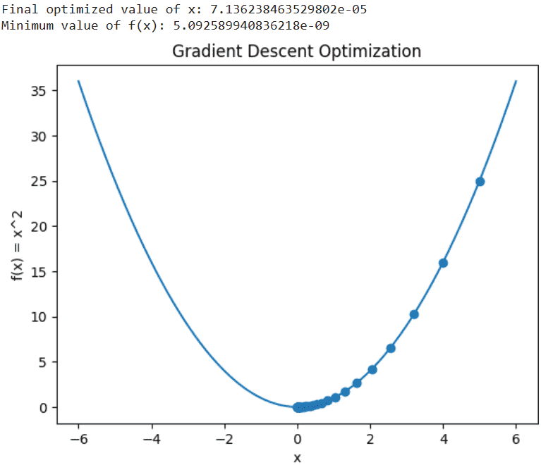
Output

**Variants of Gradient Descent

• **Batch Gradient Descent: Uses the entire dataset to compute the gradient and update parameters. It is stable but can be slow for very large datasets.
• **Stochastic Gradient Descent (SGD): Updates model parameters using one training example at a time. It requires less computation and works well for large datasets.
• **Mini Batch Gradient Descent:Updates parameters using small batches of data instead of the entire dataset. It balances speed and stability and is widely used to train deep learning models.

2. Stochastic Optimization Techniques

Stochastic optimization techniques use randomness in the optimization process to explore the search space more effectively. They are useful for solving complex problems where traditional optimization methods may get stuck in local minima.

• **Simulated Annealing: It is an optimization algorithm inspired by metallurgy. It escapes local minima by gradually reducing randomness to find near optimal solutions.
• **Random Search****:** A simple method that randomly selects points in the search space and evaluates them. It is surprisingly effective for high dimensional optimization problems.

3. Evolutionary Algorithms

Evolutionary Algorithms are optimization methods inspired by natural selection. They work by evolving a group of candidate solutions over multiple generations to find good or near optimal solutions for complex problems. Main components of Evolutionary Algorithms are:

• **Population: A group of possible solutions.
• **Fitness Function: Measures how good each solution is.
• **Selection: Chooses the better solutions for reproduction.
• **Genetic Operators: Create new solutions using crossover and mutation.
• **Termination: Stops the process after a condition is met.

**Techniques in Evolutionary Algorithms

**1. Genetic Algorithms

Genetic Algorithms are optimization methods that evolve a population of solutions using selection, crossover and mutation.

• Start with randomly generated solutions
• Select the best solutions based on fitness
• Create new solutions through crossover and mutation
• Repeat the process for several generations

**2. Differential Evolution (DE)

Differential Evolution is a population based stochastic optimization technique that evolves candidate solutions using vector differences. It is effective for continuous, high dimensional and non convex optimization problems.

• Starts with a population of candidate solutions within defined bounds.
• For each target vector, generates a mutant vector using three distinct population members with the formula:

mutant = a +F .(b -c), where F is a scaling factor controlling variation

• Creates a trial vector by mixing the target and mutant vectors based on a crossover rate (CR).
• Replaces the target vector with the trial vector if it improves fitness and repeats the process for a fixed number of generations.

4. Metaheuristic Optimization

Metaheuristic optimization algorithms are high level methods used to solve complex optimization problems by exploring large search spaces. They help find near optimal solutions without using gradient information.

**Common Techniques

**1. Tabu Search (TS)

Tabu Search improves local search by using memory to avoid revisiting recently explored solutions and helps escape local optima.

• Uses a tabu list to avoid repeating recent solutions.
• Allows better solutions using aspiration rules.
• Explores new areas while improving good solutions.

**2. Iterated Local Search (ILS)

Iterated Local Search is another strategy for enhancing local search but unlike Tabu Search, it does not use memory structures. It relies on repeated application of local search, combined with random changes to escape local minima and continue the search.

• Starts with a local search to find a good solution.
• Applies small changes to escape local minima.
• Repeats the process to improve the solution.

5. Swarm Intelligence Algorithms

Swarm intelligence algorithms are inspired by the collective behaviour of natural systems such as bird flocks and ant colonies. These algorithms use multiple agents that cooperate and share information to search for good solutions.

There aretwo of the widely applied algorithms in swarm intelligence:

**1. Particle Swarm Optimization (PSO)

Particle Swarm Optimization (PSO) is a population based algorithm inspired by the social behaviour of birds and fish. Each particle represents a potential solution and moves through the search space by combining its own experience with that of the swarm.

• Particles update their velocity based on personal best and global best solutions.
• Their position is updated using the new velocity.
• Over iterations, particles move toward better solutions.

**2. Ant Colony Optimization (ACO)

Ant Colony Optimization ACO is inspired by ant foraging behaviour. Ants find shortest paths by depositing pheromones, which guide other ants toward better solutions over iterations.

• Each ant builds a path by choosing options based on pheromone strength.
• Pheromones evaporate over time and are reinforced on better paths.
• Over iterations, ants converge toward the shortest path.

6. Optimization Techniques in Deep Learning

Deep learning models often contain many parameters, making optimization important for efficient training. Different optimization techniques help models learn faster and improve prediction performance.

**Common optimizers used in Neural Networks are:

• **RMSProp:Adjusts the learning rate for each parameter using a moving average of squared gradients, which helps stabilize training and improves convergence.
• **Adam:Combines ideas from momentum and RMSProp by maintaining moving averages of gradients and their squares. It adapts learning rates for each parameter and is widely used for training deep learning models.

7. Hyperparameter Optimization

Hyperparameter optimization is the process of selecting the best hyperparameter values to improve a machine learning model’s performance. These parameters are not learned from data but strongly affect accuracy, efficiency and generalization.

• **Grid Search:Tests all possible combinations of predefined hyperparameter values to find the best one, but it can be computationally expensive.
• **Random Search****:** Randomly selects hyperparameter values from a defined range. It is faster and often works well for large or high dimensional search spaces.

Second order Algorithms

Second order optimization algorithms use both the gradient and second derivative of the loss function to update parameters more accurately. They often converge faster than first order methods but are computationally more expensive.

**1. Newton Method

Newton’s Method is an optimization technique that uses both the gradient and second derivative of a function to update parameters more accurately and reach the minimum faster than basic gradient based methods.

• Calculate the gradient (first derivative) of the function at the current point.
• Compute the Hessian matrix (second derivative) to understand the curvature.
• Update parameters using:

\theta_{\text{new}} = \theta_{\text{old}} - H^{-1} \cdot \nabla f(\theta_{\text{old}})

• Repeat the process until the change in parameters is very small or convergence is reached.

**Implementation

• **Defines the function and its derivatives: Specifies the function along with its first and second derivatives.
• **Applies Newton’s Method: Starts from an initial value and repeatedly updates it using gradient and curvature information.
• **Checks convergence: Stops when the update becomes very small or when the maximum number of iterations is reached.
• **Visualizes the result: Plots the function and highlights the stationary point found by the algorithm. Python `

import numpy as np import matplotlib.pyplot as plt

def f(x): return x3 - 2*x2 + 2

def f_prime(x): return 3x**2 - 4x

def f_double_prime(x): return 6*x - 4

def newtons_method(f_prime, f_double_prime, x0, tol=1e-6, max_iter=100): x = x0 for i in range(max_iter): second_derivative = f_double_prime(x) if second_derivative == 0: print("Zero second derivative. Stopping at iteration", i) break step = f_prime(x) / second_derivative if abs(step) < tol: print(f"Converged after {i+1} iterations") break x -= step return x, f(x)

x0 = 3.0
tol = 1e-6
max_iter = 100 result, f_val = newtons_method(f_prime, f_double_prime, x0, tol, max_iter) print("Stationary point at x =", result) print("Function value at this point f(x) =", f_val) x_vals = np.linspace(-1, 4, 500) y_vals = f(x_vals)

plt.figure(figsize=(8,5)) plt.plot(x_vals, y_vals, label="f(x) = x³ - 2x² + 2", color='blue') plt.scatter(result, f_val, color='red', zorder=5, label="Stationary Point") plt.title("Newton's Method Optimization") plt.xlabel("x") plt.ylabel("f(x)") plt.grid(True) plt.legend() plt.show()

`

**Output:

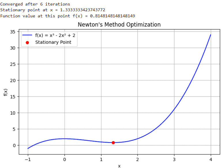
Newton Method Optimization

**2. Quasi-Newton Methods

Quasi-Newton methods are optimization algorithms that find local minima using gradient information and an approximation of the function’s curvature. Instead of computing the Hessian matrix directly, they estimate it, making the optimization process faster and more efficient.

• **Avoid full Hessian computation: Reduces computational cost.
• **Approximate curvature: Uses gradient information to estimate second order behaviour.
• **Faster convergence: Often converges faster than basic gradient descent.

**Quasi-Newton Variants

• **BFGS (Broyden-Fletcher-Goldfarb-Shanno): Estimates the Hessian matrix using gradient updates and improves it iteratively, achieving fast convergence without computing the Hessian directly.
• **L-BFGS (Limited-memory BFGS): A memory efficient version of BFGS that stores only a few past updates, making it suitable for large scale optimization problems.

3. Constrained Optimization

Constrained optimization deals with optimizing an objective function while satisfying certain restrictions or constraints. These constraints can be equality or inequality conditions and specialized methods help find optimal solutions that respect them.

• **Lagrange Multipliers:Introduce additional variables called multipliers to convert a constrained problem with equality constraints into an unconstrained one.
• **KKT (Karush-Kuhn-Tucker) Conditions: Extend Lagrange multipliers to handle both equality and inequality constraints and provide conditions for optimal solutions.

4. Bayesian Optimization

Bayesian optimization is a probabilistic method used to optimize expensive or complex functions. It builds a surrogate model of the objective function and uses past evaluations to decide where to search next.

• **Uses past evaluations: Guides the search using information from previously tested points.
• **Sample efficient: Requires fewer function evaluations than methods like Grid Search or Random Search.
• **Balances exploration and exploitation: Searches new areas while focusing on promising regions.

Limitations

• **Non-Convexity: Many loss functions have multiple local minima, making it difficult to find the global optimum.
• **High Dimensionality: Large parameter spaces increase computational complexity.
• **Overfitting: Poor optimization may cause models to memorize training data instead of generalizing.
• **Computational Cost: Some methods require expensive calculations that do not scale well for large datasets.
• **Hyperparameter Sensitivity: Performance depends on properly tuning parameters like learning rate.