Optimization in SciPy (original) (raw)
SciPy is a Python library that is available for free and open source and is used for technical and scientific computing. It is a set of useful functions and mathematical methods created using Python's NumPy module.
Features of SciPy:
- Creating complex programs and specialized applications is a benefit of building SciPy on Python.
- SciPy contains varieties of sub-packages that help to solve the most common issue related to Scientific Computation.
- SciPy users benefit from the inclusion of new modules created by programmers all around the world in a variety of software-related fields.
- Easy to use and understand as well as fast computational power.
- It can operate on an array of NumPy libraries.
Sub-packages of SciPy:
| Packages | Description |
|---|---|
| scipy.io | File input/output |
| scipy.special | Special Function(airy, elliptic, bessel, gamma, beta, etc) |
| scipy.linalg | Linear Algebra Operation |
| scipy.interpolate | Interpolation |
| scipy.optimize | Optimization and fit |
| scipy.stats | Statistics and random numbers |
| scipy.integrate | Numerical Integration |
| scipy.fftpack | Fast Fourier transforms |
| scipy.signal | Signal Processing |
| scipy.ndimage | Image manipulation |
In this article, we will learn the scipy.optimize sub-package.
This package includes functions for minimizing and maximizing objective functions subject to given constraints. Let's understand this package with the help of examples.
SciPy - Root Finding
func : callable
The function whose root is required. It must be a function of a single variable of the form f(x, a, b, c, . . . ), where a, b, c, . . . are extra arguments that can be passed in the args parameter.
x0 : float, sequence, or ndarray
Initial point from where you want to find the root of the function. It will somewhere near the actual root. Our initial guess is 0.
Find the smallest positive root of the function f(x) = x3 - 2x + 0.5 .
Import the optimize.newton package using the below command. Newton package contains a function that will calculate the root using the Newton Raphson method. Define a function for the given objective function. Use the newton function. This function will return the result object which contains the smallest positive root for the given function f1.
Python3 `
from scipy.optimize import newton
objective function
def f1(x): return xxx - 2*x + 0.5
newton function will return the root.
print(newton(func2, 0))
`
Output:
0.25865202250415226
SciPy - Linear Programming
Maximize: Z = 5x + 4y
Constraints:
- 2y ≤ 50
- x + 2y ≤ 25
- x + y ≤ 15
- x ≥ 0 and y ≥ 0
Import the optimize.linprog module using the following command. Create an array of the objective function's coefficients. Before that convert the objective function in minimization form by multiplying it with a negative sign in the equation. Now create the two arrays for the constraints equations. One array will be for left-hand equations and the second array for right-hand side values.
Python3 `
from scipy.optimize import linprog
Objective function's Coefficient matrix
obj = [-5, -4]
Constraints Left side x and y Coefficient matrix
lhs_ineq = [[0, 2], # 0x1 + 2x2 [1, 2], # x1 + 2x2 [1, 1]] # 1x1 + 1x2
right side values matrix
rhs_ineq = [50, # ......<= 50 25, # ......<= 25 15] # ..... <= 15
`
Use the linprog inbuilt function and pass the arrays that we have created an addition mention the method.
Python3 `
Inbuilt function will
solve the problem optimally
passing the each coefficient's Matrices
opt = linprog(c=obj, A_ub=lhs_ineq, b_ub=rhs_ineq, method="highs")
printing the solution
print(opt)
`
Output:
con: array([], dtype=float64) crossover_nit: 0 eqlin: marginals: array([], dtype=float64) residual: array([], dtype=float64) fun: -75.0 ineqlin: marginals: array([-0., -0., -5.]) residual: array([50., 10., 0.]) lower: marginals: <MemoryView of 'ndarray' at 0x7f41289de040> residual: array([15., 0.]) message: 'Optimization terminated successfully.' nit: 1 slack: array([50., 10., 0.]) status: 0 success: True upper: marginals: <MemoryView of 'ndarray' at 0x7f4128a56d40> residual: array([inf, inf]) x: array([15., 0.])
This function will return an object that contains the optimal answer for the given problem.
SciPy - Assignment Problem
A city corporation has decided to carry out road repairs on main four arteries of the city. The government has agreed to make a special grant of Rs. 50 lakh towards the cost with a condition that repairs are done at the lowest cost and quickest time. If the conditions warrant, a supplementary token grant will also be considered favourably. The corporation has floated tenders and five contractors have sent in their bids. In order to expedite work, one road will be awarded to only one contractor.
Cost of Repairs ( Rs in lakh) Contractors R1 R2 R3 R4 R5 C1 9 14 19 15 13 C2 7 17 20 19 18 C3 8 18 21 18 17 C4 10 12 18 19 18 C5 10 15 21 16 15 Find the best way of assigning the repair work to the contractors and the costs. If it is necessary to seek supplementary grants,what should be the amount sought?
In this code, we required the NumPy array so first install the NumPy module and then import the required modules. Create a multidimensional NumPy array of given data. Use the optimize.linear_sum_assignment() function. This function returns two NumPy arrays (Optimal solution) - one is the row ( Contactors) and the second is the column ( Corresponding Repair Cost).
Python3 `
Import numpy module
import numpy as npy
Import linear_sum_assignment
from scipy.optimize import linear_sum_assignment
Cost_Matrix of the given data
cost_matrix = npy.array([[9, 14, 19, 15, 13], [7, 17, 20, 19, 18], [8, 18, 21, 18, 17], [10, 12, 18, 19, 18], [10, 15, 21, 16, 15]])
Extracting the optimal assignments for
contractors and corresponding Repair Cost
r, c = linear_sum_assignment(cost_matrix)
`
Use the sum() function and calculate the total minimum optimal cost.
Python3 `
Contactors
print(r)
Repair costs
print(c)
Printing the final minimal optimal cost
print(cost_matrix[r, c].sum())
`
Output:
[0 1 2 3 4] [4 0 2 1 3] 69
How the assignment will be done can be concluded below from the obtained data.
- Contractor C1 will assign road 1 with a repair cost of 13Rs Lakh.
- Contractor C2 will assign road 2 with a repair cost of 7RS lakh.
- Contractor C3 will assign road 3 with a repair cost of 21RS lakh.
- Contractor C4 will assign road 4 with a repair cost of 12RS lakh.
- Contractor C5 will assign road 5 with a repair cost of 16RS lakh.
Hence Final Minimal cost will be,
13 + 7 + 21 + 12 + 16 = Rs. 69 lakh.
SciPy - Minimize
Broyden-Fletcher-Goldfarb-Shanno ( BFGS )
This algorithm deals with the Minimization of a scalar function of one or more variables. The BFGS algorithm is one of the most widely used second-order algorithms for numerical optimization, and it is frequently used to fit machine learning algorithms such as the logistic regression algorithm.
Objective Function:
- z = sin( X ) + cos( Y )
Python3 `
importing the module
import numpy as np from scipy.optimize import minimize
BFGS Algorithm -
define the objective function
def obj(xy): x, y = xy return np.sin(x)*np.cos(y)
using the method = 'BFGS'
and (2,-5) initial point
res = minimize(obj, (2, -5), method='BFGS')
printing the result
print(res)
`
Output:
**fun: -0.999999999999904**hess_inv: array([[ 1.01409071, -0.00302069], [-0.00302069, 1.00066793]]) jac: array([-4.24683094e-07, 9.68575478e-08]) message: 'Optimization terminated successfully.' nfev: 24 nit: 6 njev: 8 status: 0 success: True x: array([ 1.5707959 , -3.14159257])
SciPy - curve_fit
Curve fitting requires that you define the function that maps examples of inputs to outputs like Machine Learning supervised learning. The mapping function can have a straight line (Linear Regression), a Curve line (Polynomial Regression), and much more. A detailed GeeksForGeeks article on Scipy Curve_fit is available here SciPy | Curve Fitting.
Python3 `
importing the module
import numpy as np import matplotlib.pyplot as plt from scipy.optimize import curve_fit
data points -
xd = np.array([-8.0, -7.0, -6.0, -5.0, -4.0, -3.0, -2.0, -1.0, 0.0, 1.0, 2.0, 3.0, 4.0, 5.0, 6.0, 7.0, 8.0])
yd = np.array([13.6, 11.1, 12.0, 14.9, 13.7, 16.1, 19.6, 17.0, 15.3, 18.4, 14.8, 11.6, 10.2, 8.9, 9.1, 3.1, 1.1])
cosine function
def fcos(p, q, r): return qnp.cos(rp)
Extracting x,y values
p0 - initial guess
x, y = curve_fit(fcos, xd, yd, p0=[19, 0.1])
print(x, y)
calling the function
fit_c = fcos(xd, x[0], x[1])
plotting the graph
plt.plot(xd, yd, 'o', label='data') plt.plot(xd, fit_c, '-', label='fit')
`
Output:
[16.45191102 0.14955689] [[1.74663622e+00 1.19187398e-02] [1.19187398e-02 2.52349161e-04]]
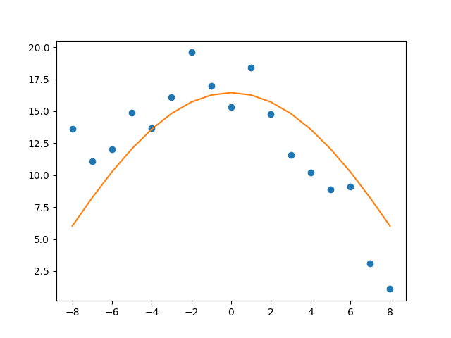
Approximate curve fitted to the input points
SciPy - Univariate Function Minimizers
Non-linear optimization with no constraint and there is only one decision variable in this optimization that we are trying to find a value for.
Python3 `
importing the module
from scipy.optimize import minimize_scalar
Objective function
def A(x): return (x - 2) * (x + 2)**2
printing the optimized result
print(minimize_scalar(A, bounds=(-5, 5), method='bounded'))
`
Output:
**fun: -9.481481481481376**message: 'Solution found.' nfev: 12 status: 0 success: True x: 0.6666668296237073
Nelder-Mead Simplex Search - Machine Learning
Noisy Optimization Problem - A noisy objective function is a function that gives different answers each time the same input is evaluated.
Python3 `
nelder-mead optimization of
noisy one-dimensional convex function
from scipy.optimize import minimize from numpy.random import randn
objective function
def A(q): return (q + randn(len(q))*0.28)**2.0
printing the optimal function
print(minimize(A, 0.5, method='nelder-mead'))
`
Output:
final_simplex: (array([[0.52539082], [0.52539063]]), array([6.79569941e-07, 9.02524100e-05])) fun: 6.795699413959474e-07 message: 'Optimization terminated successfully.' nfev: 47 nit: 18 status: 0 success: True x: array([0.52539082])