Orthogonal distance regression using SciPy (original) (raw)
Last Updated : 23 Jul, 2025
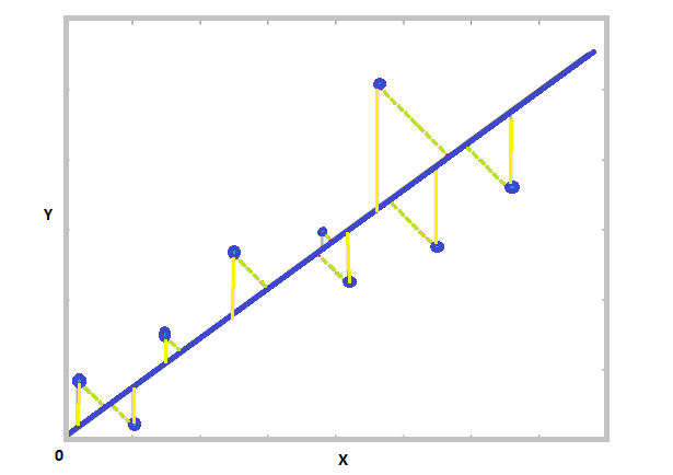
Orthogonal Distance Regression (ODR) is a powerful statistical technique used to fit a model to data when both independent (X) and dependent (Y) variables are subject to error. Unlike traditional Ordinary Least Squares (OLS), which assumes that only the dependent variable has measurement errors, ODR accounts for errors in both directions, making it ideal for scientific and engineering data where all measurements can be noisy.
Why Use ODR Instead of OLS?
In many real-world scenarios, both the independent variable (X) and the dependent variable (Y) may be affected by measurement errors. In such cases, ODR becomes more suitable because it:
- Accounts for errors in both X and Y
- Provides a more geometrically accurate fit
- Is capable of handling non-linear models
Mathematical Formulation
The objective function minimized in ODR is:
\sum_{i=1}^{n} \left[ \frac{(y_i - \alpha - \beta x_i)^2}{\eta} + (x_i - X_i)^2 \right]
Where:
- 𝑦𝑖: observed dependent variable
- 𝑥𝑖: true (unknown) value of the independent variable
- 𝑋𝑖: observed value of the independent variable
- \alpha,\beta: regression coefficients (intercept and slope)
- \eta : weighting factor between Y and X errors
And the weighting factor \eta is defined as:
\eta = \frac{\sigma_\xi^2}{\sigma_\mu^2}
Where:
- \sigma_\xi^2: variance of error in the dependent variable (Y-axis)
- \sigma_\mu^2: variance of error in the independent variable (X-axis)
Implementation in SciPy
SciPy provides the scipy.odr module to implement ODR using the ODRPACK library, a well-established FORTRAN-77 based package. SciPy wraps this functionality in an object-oriented interface for ease of use.
Step-by-Step Approach
- Import required libraries
- Create input data arrays (feature, target)
- Define a model function (e.g., linear)
- Use odr.Model() to wrap the model function
- Wrap data using odr.Data()
- Create and configure odr.ODR() instance
- Run the regression using .run()
- Display results with .pprint() Python `
import numpy as np import matplotlib.pyplot as plt from scipy import odr
x = np.arange(1, 11) np.random.shuffle(x) y = np.array([0.65, -0.75, 0.90, -0.5, 0.14, 0.84, 0.99, -0.95, 0.41, -0.28])
def model_fn(p, x): m, c = p return m * x + c
model = odr.Model(model_fn) data = odr.Data(x, y) odr_run = odr.ODR(data, model, beta0=[0.2, 1.0]) res = odr_run.run() res.pprint()
`
**Output
Beta: [ 0.11545417 -0.48999795]
Beta Std Error: [0.07475684 0.46382517]
Beta Covariance: [[ 0.01228991 -0.06759452]
[-0.06759452 0.4731028 ]]
Residual Variance: 0.45472947791705537
Inverse Condition #: 0.06923218954368635
Reason(s) for Halting:
Sum of squares convergence