Principal Component Analysis with R Programming (original) (raw)
Last Updated : 30 Apr, 2026
Principal Component Analysis (PCA) is a machine learning technique used to reduce the dimensionality of large datasets while preserving as much information as possible. It transforms correlated variables into a smaller set of uncorrelated variables called principal components, making complex datasets easier to understand and visualize. PCA is widely used in Exploratory Data Analysis (EDA) and as a preprocessing step in predictive modeling.

Principal Component Analysis (PCA)
PCA transforms the original variables into new components, where each component captures the maximum remaining variance in the data.
- The first principal component (PC1) captures the maximum variance in the dataset and represents the direction of greatest variability.
- The second principal component (PC2) captures the next highest variance and is uncorrelated (orthogonal) to PC1.
- Each subsequent component (PC3, PC4 and so on) captures the remaining variance while remaining orthogonal to all previous components.
How Principal Component Analysis (PCA) Works in R
PCA converts correlated numerical variables into a smaller set of uncorrelated components using linear algebra methods. In R, it is performed using the functions prcomp() or princomp(), which calculate the principal components using SVD or eigendecomposition.
Step 1: Standardize the Data
PCA is sensitive to scale. If variables are measured in different units (e.g., income and age), features with larger scales may dominate the results. Therefore, data is usually standardized before applying PCA.
Standardization is done using:
Z=\frac{X-\mu}{\sigma}
where
- \mu: mean of the feature
- \sigma: standard deviation of the feature
Step 2: Compute the Covariance (or Correlation) Matrix
After scaling, PCA examines relationships between variables by computing the covariance matrix (or correlation matrix if standardized).
Covariance between two variables x1 and x2 is:
cov(x_1, x_2) = \frac{\sum_{i=1}^{n}(x_{1i} - \bar{x}_1)(x_{2i} - \bar{x}_2)}{n - 1}
The covariance matrix is symmetric and shows how variables vary together:
- **Positive covariance: variables increase together
- **Negative covariance: one increases while the other decreases
- **Zero: no linear relationship
Step 3: Compute Eigenvectors and Eigenvalues
PCA then calculates:
- **Eigenvectors: directions of maximum variance (principal components)
- **Eigenvalues: amount of variance explained by each component
AX=\lambda X
where
- A: covariance matrix
- X: eigenvector
- \lambda: eigenvalue
Step 4: Select the Principal Components
- Principal components are ranked based on their eigenvalues (amount of variance explained).
- PC1 captures the highest variance in the dataset.
- PC2 captures the second highest variance and is orthogonal to PC1.
- Subsequent components continue in decreasing order of explained variance.
Step 5: Transform the Data
Finally, the original data is projected onto the selected principal components. This creates a new dataset in a lower-dimensional space while preserving most of the important information.
Z = X W
Where:
- X: standardized data
- W: matrix of selected eigenvectors
- Z: transformed dataset (principal component scores)
Step By Step Implementation
We will perform Principal Component Analysis (PCA) on the mtcars dataset to reduce dimensionality, visualize the variance and explore the relationships between different car attributes.
Step 1: Installing and Loading the Required Packages
We will install and load the necessary packages.
- **install.packages(): Installs the package.
- **library(): Loads the package. R `
install.packages("dplyr") library(dplyr)
`
Step 2: Loading the Dataset
The mtcars dataset is a built in data set in R. It contains data on fuel consumption and various performance and design aspects of 32 cars. This dataset has 11 variables, including miles per gallon (mpg), horsepower and weight.
- **str(): give the structure of the dataset R `
str(mtcars)
`
**Output:
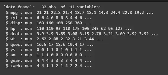
mtcars dataset
Step 3: Performing PCA
To perform PCA, we use the prcomp() function. It is used to scale and center the data before applying PCA since PCA is based on distance measures and scaling ensures that all variables are treated equally.
- **prcomp(): Performs Principal Component Analysis.
- **scale. = TRUE: Scales the data before applying PCA.
- **center = TRUE: Centers the data before applying PCA (subtracts the mean).
- **retx = TRUE: Returns the transformed data (principal components). R `
my_pca <- prcomp(mtcars, scale. = TRUE, center = TRUE, retx = TRUE) names(my_pca)
`
**Output:
'sdev''rotation''center''scale''x'
Step 4: Summary of PCA Results
We will summaries the PCA model to understand how much variance is captured by each principal component.
- **summary(): Summarizes the PCA results, including the proportion of variance explained by each principal component. R `
summary(my_pca)
`
**Output:
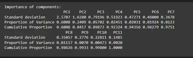
Summary of PCA Results
Step 5: Principal Component Loadings
We will see the weights (loadings) of each variable in the principal components.
- **my_pca$rotation: Shows the loadings (coefficients) of the principal components. R `
my_pca$rotation[1:5, 1:4]
`
**Output:
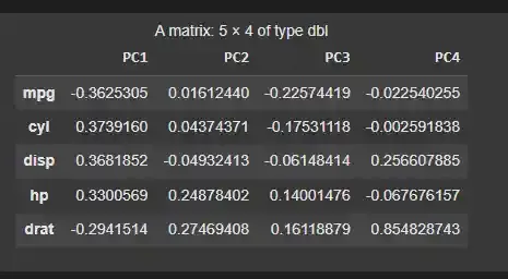
Principal Component Loadings
Step 6: Principal Components Scores
We will now inspect the scores (values of the observations on each principal component).
- **my_pca$x: Provides the transformed data in terms of principal components (scores).
- **head(): displays the first few rows R `
head(my_pca$x)
`
**Output:

Principal Components Scores
Step 7: Visualizing the Principal Components
We will use a biplot to visualize the principal components and their contributions to the overall variance.
- **biplot(): Plots the principal components and their relationships.
- **scale = 0: Ensures that arrows are scaled to represent loadings. R `
biplot(my_pca, main = "Biplot of Principal Components", scale = 0)
`
**Output:
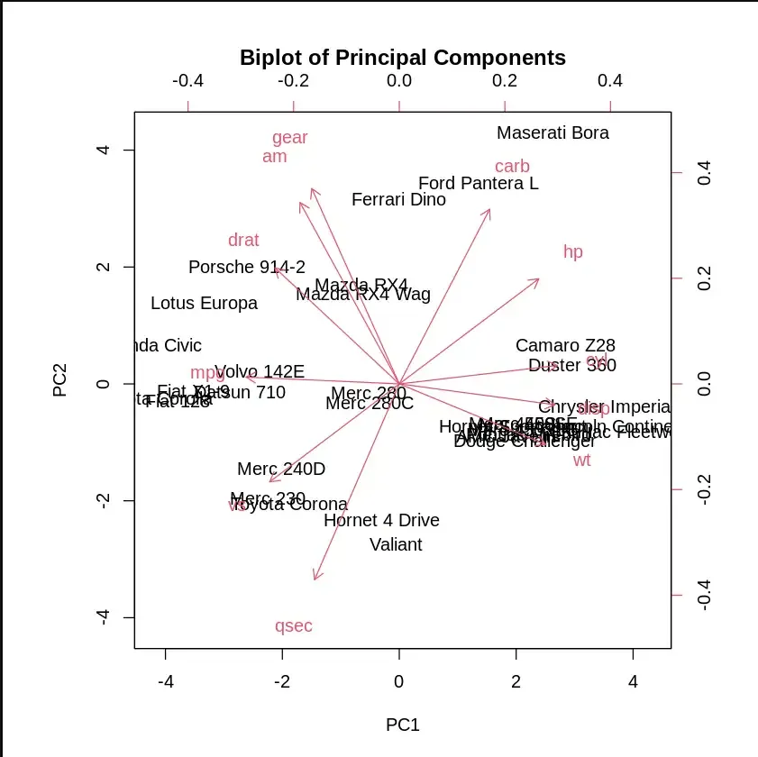
Visualizing the Principal Components
Step 8: Computing Standard Deviation and Variance
We will now compute Standard Deviation and Variance
- **my_pca$sdev: Displays the standard deviation of each principal component.
- **my_pca.var <- my_pca$sdev^2: Computes the variance of each component. R `
my_pca.var <- my_pca$sdev^2
cat("Standard Deviation :",my_pca$sdev,"\n") cat("Variance :",my_pca.var,"\n")
`
**Output:
Standard Deviation : 2.570681 1.628026 0.7919579 0.5192277 0.4727061 0.4599958 0.3677798 0.350573 0.2775728 0.2281128 0.1484736
Variance : 6.6084 2.650468 0.6271973 0.2695974 0.2234511 0.2115961 0.135262 0.1229014 0.07704665 0.05203544 0.02204441
Step 9: Proportion of Variance Explained
We calculate the proportion of variance for each component and visualize it using a scree plot to see how much variance each principal component explains.
- **plot(): Plots the proportion of variance explained by each principal component.
- **xlab : Label for the x-axis.
- **ylab: Label for the y-axis.
- **ylim = c(0, 1): Sets the y-axis limits from 0 to 1.
- **type = "b": Plots both points and lines. R `
propve <- my_pca.var / sum(my_pca.var)
plot(propve, xlab = "Principal Component", ylab = "Proportion of Variance Explained", ylim = c(0, 1), type = "b", main = "Scree Plot")
`
**Output:
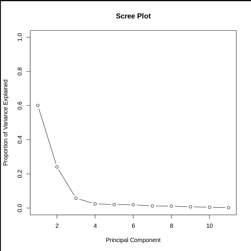
Proportion of Variance Explained
Step 10: Cumulative Proportion of Variance
We can see the cumulative variance explained by the components.
- **cumsum(): Calculates the cumulative sum of variance explained by the components.
- **plot(): Plots the cumulative proportion of variance. R `
plot(cumsum(propve), xlab = "Principal Component", ylab = "Cumulative Proportion of Variance Explained", ylim = c(0, 1), type = "b")
`
**Output:
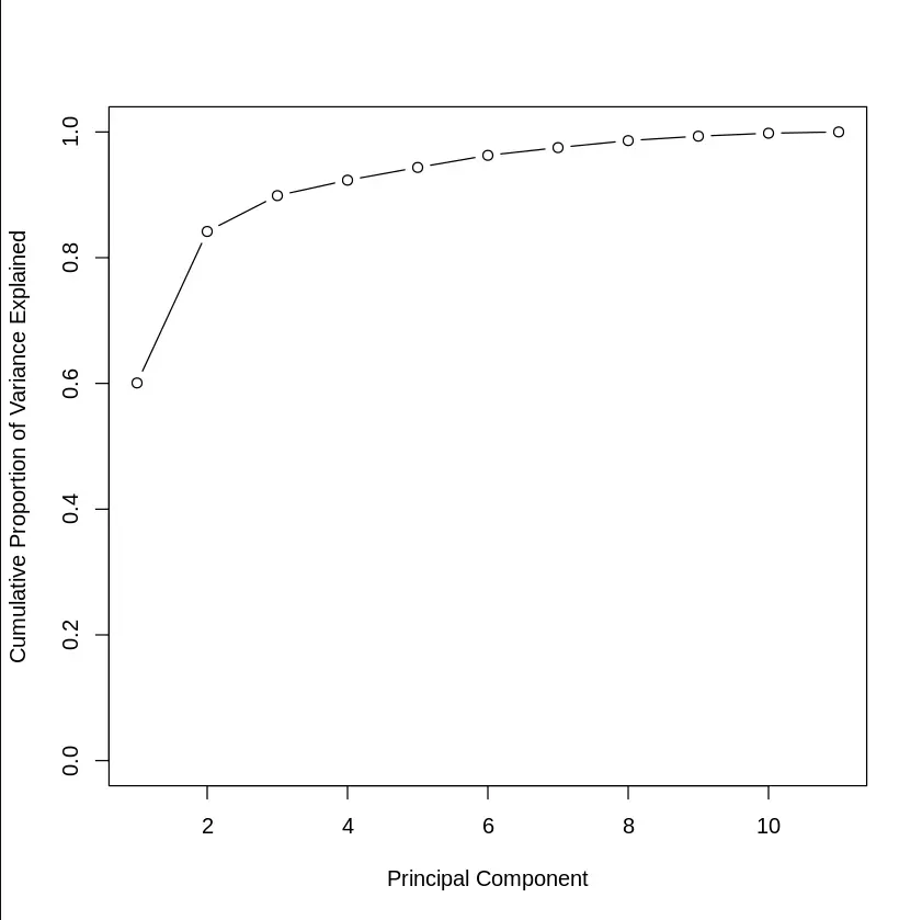
Cumulative Proportion of Variance
Step 11: Choosing Top Principal Components
We can identify the smallest number of principal components that explain at least 90% of the variance.
- **which(cumsum(propve) >= 0.9)[1]: Finds the smallest number of principal components that explain at least 90% of the variance. R `
which(cumsum(propve) >= 0.9)[1]
`
**Output:
4
Step 12: Predicting with Principal Components
We can now use the first few principal components to predict another variable. For example, predicting disp (displacement) from the top 4 principal components.
- **data.frame(): Creates a new data frame, combining the original variable (disp) with the first 4 principal components. R `
train.data <- data.frame(disp = mtcars$disp, my_pca$x[, 1:4])
head(train.data)
`
**Output:
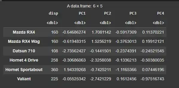
Predicting with Principal Components
Step 13: Building a Decision Tree
Next, we can use the rpart package to build a decision tree model to predict disp using the first four principal components.
- **rpart(): Fits a decision tree model.
- **disp ~ .: Formula for predicting disp using all other variables (principal components in this case).
- **data = train.data: Specifies the data to use for fitting the model.
- **method = "anova": Specifies that the model is for regression.
- **rpart.plot(): Plots the decision tree. R `
install.packages("rpart") install.packages("rpart.plot")
library(rpart) library(rpart.plot)
rpart.model <- rpart(disp ~ ., data = train.data, method = "anova")
rpart.plot(rpart.model)
`
**Output:
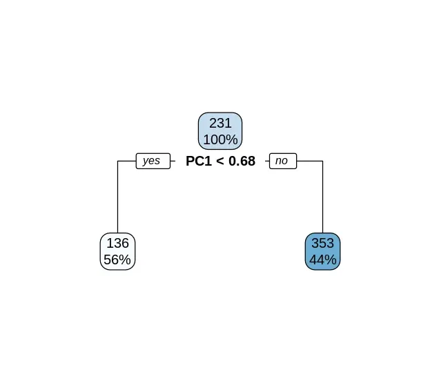
Building a Decision Tree