Ridge Regression in R Programming (original) (raw)

Last Updated : 8 Jul, 2025

Ridge Regression is a regularized version of linear regression that aims to address the problem of multicollinearity and overfitting in linear models. It modifies the standard least squares loss function by adding a penalty term that is proportional to the square of the magnitude of the coefficients (also called L2 norm).

Ridge Regression Line

A ridge regression line represents the linear relationship between predictors and the response, while shrinking large coefficient estimates to stabilize the model. As lambda increases:

• Coefficient values shrink closer to zero.
• Model becomes more stable and less likely to overfit.

Assumptions of Ridge Regression

Ridge Regression assumes the following:

• **Linear relationship: Between predictors and target.
• **No perfect multicollinearity: It tolerates multicollinearity, but not exact correlation.
• **Homoscedasticity: Constant error variance across predictors.
• **Normal error terms: Residuals are normally distributed.
• **Independent residuals: Errors are uncorrelated.

Mathematical Formulation

The cost function for Ridge Regression is:

\text{Cost} = \sum_{i=1}^{n} (y_i - \hat{y}_i)^2 + \lambda \sum_{j=1}^{m} \theta_j^2

**Where:

• y_i: actual target value for the _iᵗʰ observation.
• \hat{y}_i: predicted value for the _iᵗʰ observation.
• \theta_j: regression coefficient for feature _j.
• \lambda: regularization parameter that controls the strength of the penalty

Implementation of Ridge Regression in R

We implement Ridge Regression using the Big Mart dataset, which includes sales and product features across 10 stores to predict product sales using L2 regularization.

1. Installing Required Packages

We install the necessary packages to preprocess data, train the ridge regression model, and visualize results.

• **data.table: used to read and manipulate large datasets efficiently.
• **dplyr: used for filtering, transforming, and joining data.
• **glmnet: used for fitting ridge and lasso regression models.
• **ggplot2: used for plotting and visualization.
• **caret: used to train and tune machine learning models.
• **xgboost: used for building tree-based ensemble models.
• **e1071: used to compute statistical measures like skewness.
• **cowplot: used to combine multiple ggplots into a single layout. R `

install.packages("data.table") install.packages("dplyr") install.packages("glmnet") install.packages("ggplot2") install.packages("caret") install.packages("xgboost") install.packages("e1071") install.packages("cowplot")

library(data.table) library(dplyr) library(glmnet) library(ggplot2) library(caret) library(xgboost) library(e1071) library(cowplot)

`

2. Loading and Combining the Dataset

We load the train and test datasets and combine them for uniform preprocessing. You can download the dataset links from here: Train.csv and Test.csv.

• **fread: used to load CSV files efficiently.
• **rbind: used to combine training and test datasets. R `

train = fread("Train.csv") test = fread("Test.csv") test[, Item_Outlet_Sales := NA] combi = rbind(train, test)

`

3. Treating Missing and Zero Values

We clean the data by filling missing values and replacing invalid entries.

• **which: used to locate missing or zero-value entries.
• **mean: used to impute missing or zero values based on group-wise average. R `

missing_index = which(is.na(combi$Item_Weight)) for(i in missing_index) { item = combi$Item_Identifier[i] combi$Item_Weight[i] = mean(combi$Item_Weight[combi$Item_Identifier == item], na.rm = T) }

zero_index = which(combi$Item_Visibility == 0) for(i in zero_index) { item = combi$Item_Identifier[i] combi$Item_Visibility[i] = mean(combi$Item_Visibility[combi$Item_Identifier == item], na.rm = T) }

`

4. Encoding Categorical Features

We convert text-based features into numeric form using label encoding and one-hot encoding.

• **ifelse: used for label encoding.
• **dummyVars: used for generating one-hot encoded features.
• **predict: used to apply the encoding transformation. R `

combi[, Outlet_Size_num := ifelse(Outlet_Size == "Small", 0, ifelse(Outlet_Size == "Medium", 1, 2))] combi[, Outlet_Location_Type_num := ifelse(Outlet_Location_Type == "Tier 3", 0, ifelse(Outlet_Location_Type == "Tier 2", 1, 2))] combi[, c("Outlet_Size", "Outlet_Location_Type") := NULL]

ohe_1 = dummyVars("~.", data = combi[, -c("Item_Identifier", "Outlet_Establishment_Year", "Item_Type")], fullRank = T) ohe_df = data.table(predict(ohe_1, combi[, -c("Item_Identifier", "Outlet_Establishment_Year", "Item_Type")])) combi = cbind(combi[, "Item_Identifier"], ohe_df)

`

5. Transforming and Scaling Features

We reduce skewness and normalize numerical variables.

• **log: used to reduce skewness of positively skewed variables.
• **preProcess: used to center and scale data.
• **predict: used to apply the scaling transformation. R `

combi[, Item_Visibility := log(Item_Visibility + 1)] num_vars = which(sapply(combi, is.numeric)) num_vars_names = names(num_vars) combi_numeric = combi[, setdiff(num_vars_names, "Item_Outlet_Sales"), with = F] prep_num = preProcess(combi_numeric, method = c("center", "scale")) combi_numeric_norm = predict(prep_num, combi_numeric) combi[, setdiff(num_vars_names, "Item_Outlet_Sales") := NULL] combi = cbind(combi, combi_numeric_norm)

`

6. Splitting the Data

We split the processed dataset back into training and test sets.

• **nrow: used to determine row limits for splitting.
• ****:= NULL**: used to remove target column from test data. R `

train = combi[1:nrow(train)] test = combi[(nrow(train) + 1):nrow(combi)] test[, Item_Outlet_Sales := NULL]

`

7. Training Ridge Regression Model

We train a Ridge Regression model using cross-validation and parameter tuning.

• **trainControl: used to define cross-validation strategy.
• **expand.grid: used to specify tuning values for lambda.
• **train: used to train the model using glmnet.
• **mean: used to calculate average RMSE.
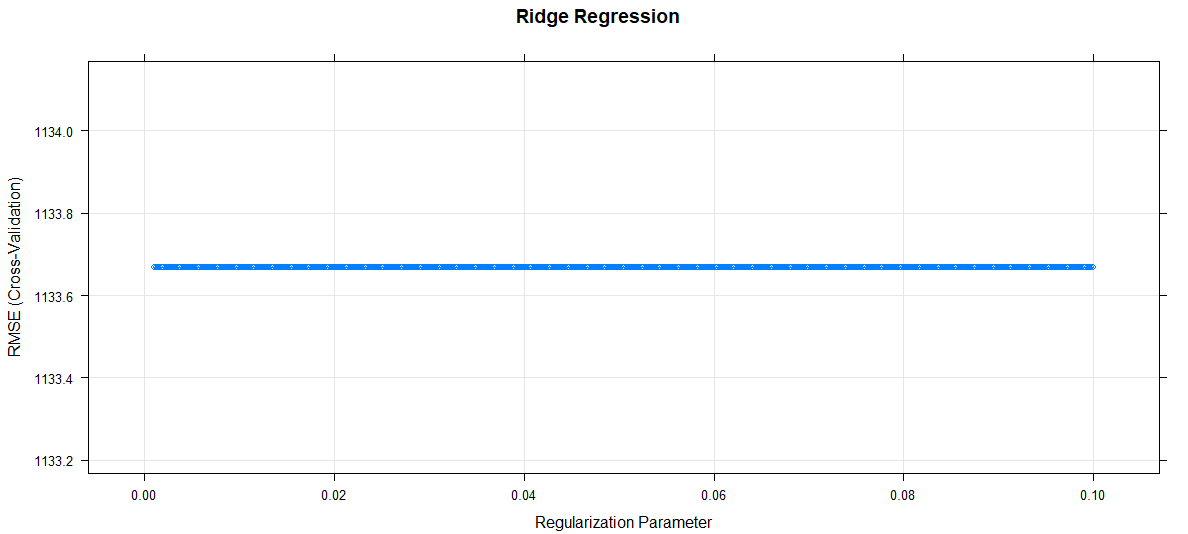
• **plot: used to visualize the model’s performance. R `

set.seed(123) control = trainControl(method = "cv", number = 5) Grid_ri_reg = expand.grid(alpha = 0, lambda = seq(0.001, 0.1, by = 0.0002)) Ridge_model = train(x = train[, -c("Item_Identifier", "Item_Outlet_Sales")], y = train$Item_Outlet_Sales, method = "glmnet", trControl = control, tuneGrid = Grid_ri_reg) cat("Mean validation test =", mean(Ridge_model$resample$RMSE)) plot(Ridge_model, main = "Ridge Regression")

`

**Output:

Mean validation test = 1133.486

Applications of Ridge Regression

• **Multicollinearity handling: Stabilizes models when predictors are highly correlated.
• **High-dimensional data: Effective when the number of features exceeds observations (e.g., genomics, text).
• **Retail sales prediction: Used to forecast product sales using multiple product/store attributes.
• **Credit risk modeling: Helps estimate default risk with many financial indicators.
• **Healthcare analytics: Predicts outcomes using numerous clinical variables.