What is the Glmnet package in R? (original) (raw)

Last Updated : 23 Jul, 2025

The glmnet package in R is used to build linear regression models with special techniques called Lasso (L1) and Ridge (L2). These techniques add a small penalty to the model to avoid making it too complex which helps prevent overfitting and makes the model work better on new data.

Regularized Regression

A type of regression that adds a penalty term to the cost function to reduce overfitting.

• **Lasso Regression: A type of regularized regression that adds an L1 penalty term to the cost function.
• **Ridge Regression: A type of regularized regression that includes an L1 penalty term in the cost function.
• **Elastic Net Regression: A type of regularized regression that includes both L1 and L2 penalty term in the cost function.

Syntax

glmnet(X, y, family = "gaussian", alpha = 1, lambda = NULL)

The main function in the glmnet package is glmnet() which fits a regularized generalized linear model. The function accepts a number of important arguments:

• **x: The matrix of predictor variables.
• **y: The response variable.
• **alpha: Declares the type of regularization (Lasso: alpha = 1, Ridge: alpha = 0, Elastic Net: 0 < alpha < 1).
• **lambda: Regularization parameter that affects the strength of the penalty.
• **family: specifies the type of response variable (e.g., Gaussian, binomial, Poisson).

Fitting a Lasso Regression Model

Lasso regression helps prevent overfitting by shrinking less important feature coefficients using an L1 penalty. We will now implement it using the glmnet package.

1. Installing and loading the glmnet package

We first install and load the glmnet package which provides tools for regularized regression.

• **install.packages("glmnet"): Installs the package from CRAN.
• **library(glmnet): Loads the package into the R session so we can use its functions. R `

install.packages("glmnet") library(glmnet)

`

2. Loading and preparing the data

We use the built-in mtcars dataset and split it into predictor and response variables.

• **data(mtcars): Loads the dataset into the environment.
• **X: A matrix of predictor variables (all columns except the first).
• **y: A response variable (miles per gallon or mpg, the first column).
• **as.matrix(): Converts the predictors to a matrix which is required by glmnet(). R `

data(mtcars)

X <- as.matrix(mtcars[, -1])

y <- mtcars[, 1]

`

3. Fitting the Lasso regression model

We now fit the Lasso model using the glmnet() function.

• **glmnet(): Fits a regularized linear model.
• **family = "gaussian": Specifies linear regression.
• **alpha = 1: Sets the model type to Lasso regression.
• **summary(): Displays a summary of the fitted model. R `

model = glmnet(X, y, family = "gaussian", alpha = 1)

summary(model)

`

**Output:

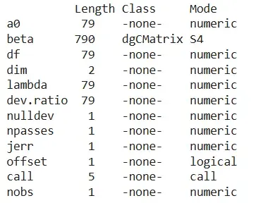
Output

4. Plotting the model

We visualize how coefficients shrink as the regularization strength increases.

• **plot(): Visualizes the coefficient paths.
• **label = TRUE: Adds variable labels to the plot. R `

plot(model, label = TRUE)

`

**Output:

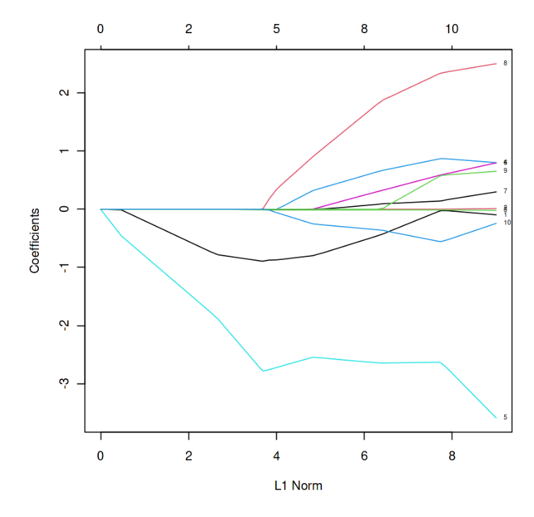
L1 Norm vs Estimated coefficients

In the above graph, each curve represents the path of the coefficients against the L1 norm as lambda varies.

5. Getting model coefficients

We extract the coefficients at a specific value of lambda.

• **coef(): Retrieves coefficients from the fitted model.
• **s: Specifies the lambda value at which to extract them. R `

coef(model, , s = 0.1)

`

**Output:

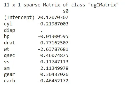
Output

6. Making predictions with the model

We use the trained model to predict response values based on the predictors.

• **predict(): Predicts response values using the model.
• **X: Matrix of predictor variables. R `

y_pred <- predict(model, X)

`

Using Cross-Validation for Lasso Model

Cross-validation helps us choose the best value of the regularization parameter lambda, improving the model’s performance and generalization.

1. Fitting a Lasso model with cross-validation

To automatically find the best lambda, we use the cv.glmnet() function which performs k-fold cross-validation on a Lasso model.

• **cv.glmnet(): Fits a Lasso model while tuning lambda through cross-validation.
• **alpha = 1: Specifies Lasso regression.
• **nfolds: Defines how many folds to use in the cross-validation.
• **summary(): Prints the structure of the fitted cross-validated model. R `

fit <- cv.glmnet(X, y, alpha = 1, nfolds = 5)

summary(fit)

`

**Output:

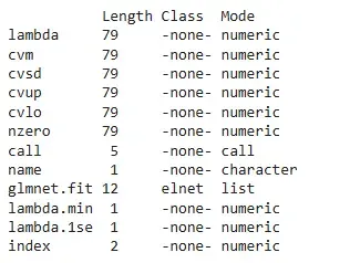
Output

2. Plotting cross-validation results

To visualize how the model performed across different lambda values, we use the plot() function.

• **plot(): Plots mean squared error for each lambda tested during cross-validation and highlights the optimal values (lambda.min, lambda.1se). R `

plot(fit)

`

**Output:

cross-validation

3. Making predictions and plotting actual vs predicted

Once the model is fitted, we use predict() to generate predictions and plot() to visually compare predicted vs actual values.

• **predict(): Uses the cross-validated model to predict the response variable.
• **plot(): Creates a scatter plot with actual values on the x-axis and predicted values on the y-axis. R `

y_pred <- predict(fit, X)

plot(y, y_pred, xlab = 'Actual', ylab = 'Predicted', main = 'Actual vs Predicted')

`

**Output:

Actual (y) vs predicted

The scatter plot shows a strong positive relationship between actual and predicted values, indicating that the Lasso model made accurate predictions.