The energetics of organic synthesis inside and outside the cell (original) (raw)
Abstract
Thermodynamic modelling of organic synthesis has largely been focused on deep-sea hydrothermal systems. When seawater mixes with hydrothermal fluids, redox gradients are established that serve as potential energy sources for the formation of organic compounds and biomolecules from inorganic starting materials. This energetic drive, which varies substantially depending on the type of host rock, is present and available both for abiotic (outside the cell) and biotic (inside the cell) processes. Here, we review and interpret a library of theoretical studies that target organic synthesis energetics. The biogeochemical scenarios evaluated include those in present-day hydrothermal systems and in putative early Earth environments. It is consistently and repeatedly shown in these studies that the formation of relatively simple organic compounds and biomolecules can be energy-yielding (exergonic) at conditions that occur in hydrothermal systems. Expanding on our ability to calculate biomass synthesis energetics, we also present here a new approach for estimating the energetics of polymerization reactions, specifically those associated with polypeptide formation from the requisite amino acids.
Keywords: hydrothermal systems, organic synthesis, biomolecule synthesis, bioenergetics, polypeptide formation
1. Introduction
It is generally accepted that organisms synthesize proteins, lipids, nucleic acids and other cellular constituents at an energetic cost. However, unless we invoke panspermia—the seeding of life from an extraterrestrial source—the prebiotic formation of the molecules that assembled into the first cells must have been thermodynamically favourable somewhere on the early Earth. In the build-up to the earliest metabolic pathways and the emergence of cells, abiotic synthesis of first simple and then more complex organic compounds was necessarily driven by natural geochemical energy sources. Since their discovery in 1977, deep-sea hydrothermal systems have been viewed as one of the most plausible environments for abiotic organic synthesis and the origin of life. Support for this theory is far-reaching and diverse, with complementary arguments from microbiology [1–3] and experimental chemistry [4–6]. A recent review of 50 years of experiments on the emergence of life concluded that ‘the best results [in these experiments] were achieved at temperatures between 60 and 90°C’, consistent with the hydrothermal system argument [7, p. 5485]. Geochemical gradients that established naturally in such systems could have enabled organic synthesis and subsequently the evolution of free-living organisms [8]. Specifically, the chemical energy required for these processes is embodied in redox disequilibria, and these are as germane for organic synthesis (and ultimately biopolymer formation) on prebiotic Earth as they are in hydrothermal ecosystems today.
Hydrothermal systems—and here we use the term in the broadest sense, to include those on land and those in deep and shallow-seafloor settings—have sparked scientific interest far beyond the emergence of metabolism and life. For example, microbial diversity studies of these systems have revealed the presence of several hundred species of thermophilic archaea and bacteria, including many deeply rooted phyla in the universal tree of life [9–13]. Aerobes and anaerobes, phototrophs and chemotrophs, and autotrophs and heterotrophs can thrive at temperatures approaching and, in some cases, exceeding 100°C [9,14–22]. There is an ever-growing number of heat-loving organisms and robust evidence of their role in many biogeochemical processes. Despite this, the energetics of organic and biomolecule synthesis at elevated temperatures and pressures have not fully entered the mainstream scientific discussion. Such investigations are paramount to a better understanding of life's limits and can be used as predictive tools to explore the Earth's (and other planetary bodies') potentially large and diverse biosphere. Here, we review the numerous thermodynamic studies on this subject, considering the formation of organic compounds both outside the cell (i.e. abiotic reactions) and inside the cell (i.e. anabolism).
It should be noted that with respect to biomass formation, thermodynamic modelling is currently limited to the level of synthesis of biomolecular monomers (i.e. amino acids, nucleotides, fatty acids, saccharides and amines). Several studies have evaluated the thermodynamic costs of synthesizing these monomers from CO2 and other inorganic nutrients [23–25], but calculating the energetics of polymerization into biopolymers such as proteins, lipids and nucleic acids has been faced with substantial hurdles. A second goal of this communication, in addition to the review component, is to advance our understanding of the thermodynamics of polypeptide and protein formation.
2. Sources of thermodynamic data for organic compounds
Two types of data provide the foundation of any effort to assess the energy associated with organic synthesis reactions, regardless of whether these are abiotic or biotic processes. On the one hand, accurate analytical data from natural systems supply concentrations of all reactants and products, as well as ionic strengths required to convert concentrations into thermodynamic activities. On the other hand, internally consistent thermodynamic data provide an independent means of assessing the extent to which constituents of natural systems depart from states of equilibrium and, therefore, represent sources of energy if reactions among them are catalysed. In this section, we review sources of internally consistent thermodynamic data for organic compounds and summarize strategies that can be used to estimate additional values of compounds of interest.
The notion that data must be internally consistent to be useful in bioenergetic calculations can be understood by reflecting on the variety of experiments that yield thermodynamic properties. Some experiments provide data that apply directly to a compound in a particular form. Examples include direct calorimetric measurements on a sample of a liquid hydrocarbon or a crystalline amino acid. Other experiments provide data on a compound during a phase transition, or during a reaction involving other compounds. One example would be measurements of the heat of solution of a liquid hydrocarbon as it dissolves into an aqueous solution. Another would be measuring the heat of combustion of a crystalline amino acid as it is oxidized into CO2, N2 and H2O vapour. In the case of direct calorimetric measurements, there is little ambiguity about how to assign the resulting thermodynamic properties. When a reaction is involved, the property obtained refers to the reaction itself, and although it must be possible to combine the properties of the constituents in the reaction to obtain the reaction property, there are many possible combinations. Using the hydrocarbon example, obtaining an enthalpy value for the aqueous form from the heat of solution measurement depends on the choice of enthalpy for the liquid form. Likewise, obtaining an enthalpy value of the amino acid from the heat of combustion measurement depends on the enthalpy values selected for the gases CO2, N2 and H2O. To maintain internal consistency, the same data for these gases would need to be used to interpret heat of combustion measurements for another amino acid. In fact, if the same data for CO2 and H2O are used to interpret heat of combustion data for the liquid hydrocarbon, then the resulting thermodynamic properties of the hydrocarbon and the amino acid would be internally consistent, and so on. This is the underlying strategy for building an internally consistent database of thermodynamic properties for any substance, which permits any imaginable reaction among those substances to be studied. Because geochemical processes involve minerals, aqueous solutions, gases, silicate melts, petroleum, organic compounds and biomolecules, geochemists have constructed fairly diverse internally consistent thermodynamic databases.
Efforts in geochemistry to build an internally consistent thermodynamic database of organic compounds began with the publication of data for about 80 aqueous species [26]. In the process, consistency of these data was established with thermodynamic data for inorganic aqueous ions and neutral solutes [27,28], as well as for minerals, gases and H2O [29]. Internal consistency was maintained as data for inorganic ions and complexes were expanded [30–35]. These efforts used the revised Helgeson–Kirkham–Flowers (HKF) equation of state for aqueous solutes [36,37]. As a consequence, it became possible to consider the effects of organic oxidation–reduction reactions on the stabilities of minerals containing iron, sulfur and other redox-sensitive elements and vice versa, at the prevailing temperatures and pressures of sedimentary basins and hydrothermal systems. Such analyses led to new ideas regarding metastable equilibrium and hydrolytic disproportionation in geochemical processes [38–41], which provided the foundation for models of abiotic organic synthesis in hydrothermal systems [42–46]. It also became possible to examine the effects of organic acid decarboxylation reactions that produce CO2 on the stabilities of carbonate minerals [41].
Early efforts focused on expanding the number and variety of organic compounds that could be included in geochemical calculations. These involved new data for aqueous aldehydes [47], small peptides [48], alkylphenols [49], aqueous mono- and dicarboxylic acids and hydroxy acids [50], aqueous metal–organic complexes involving organic acids [51–53], chloroethylenes [54] and carbohydrates [55]. These developments depended on using experimental data to generate correlation algorithms that permit estimation of data that have not been measured directly, and were extended to thiols [56] and organic sulfides [57]. Additional correlations built on regression of experimental data permitted estimation of parameters for the revised-HKF equation of state [58].
At the time, the existing high-temperature–pressure thermodynamic data for aqueous organic compounds were relatively limited. This meant that the applicability of correlation algorithms was constrained to compounds with similar molecular structures. This problem was overcome by the introduction of group contribution estimation methods for families of aqueous organic compounds, including amino acids and unfolded proteins [59–61], and for pure hydrocarbons, carboxylic acids, amino acids, thiols, alcohols and other organic compounds such as solids, liquids or gases [62]. In the development of group contribution methods, experimental data are regressed to obtain contributions from functional groups of organic compounds. These functional-group contributions can then be summed to estimate data and equation of state parameters for individual compounds. The result is that a greater number and variety of organic compounds can be included in thermodynamic calculations. As an example, data for amino acids as pure solids and as aqueous solutes were combined to calculate solubilities as functions of pH at elevated temperatures and pressures [63]. The group contribution approach for pure compounds was extended to include isoprenoids, hopanes, steranes, polycyclic aromatic compounds and a wide variety of S-bearing organic compounds [64,65].
Subsequent developments in group contribution methods for estimating thermodynamic properties of aqueous organic compounds included alkanes, cycloalkanes and aromatic hydrocarbons [66,67], alcohols and ketones [68], esters [69], S-bearing compounds [70], ethers [71] and nitriles [72]. These efforts produced widely applicable but somewhat less precise first-order group contribution methods, and more highly accurate but less inclusive second-order methods that take into account interactions among functional groups. Results of group contribution estimates are compared with experimental data for dozens of aqueous solutes at the ORCHYD website (orchyd.asu.edu; [73]). At nearly the same time, progress was made in extending group contribution estimation procedures to biomolecules, including a new take on amino acids, polypeptides and unfolded proteins [74], nucleic-acid bases, nucleotides and nucleosides [75], and magnesium complexes of adenosine nucleotides, as well as oxidized and reduced nicotinamide adenosine dinucleotides (NAD) and NAD-phosphates [76]. Internally consistent data and group contribution estimation methods for crystalline forms of many of the same compounds can be found in the latter publications, and internally consistent thermodynamic data for crystalline peptides were also contributed recently [77].
It is now possible to include organic compounds of increasing complexity from methane to proteins in geochemical calculations. The ability to include biomolecules, in particular, is permitting novel perspectives on how microbes interact with their environment, and how biochemistry operates when constrained by geochemistry. A new analysis provides the energetics associated with the degradation of organic compounds and offers thermodynamic explanations for why certain organic compounds persist in sediments, whereas others are rapidly transformed by microbial processes [78]. This approach permits the explicit inclusion of thermodynamic properties of complex organic compounds in kinetic models of organic compound degradation (see also [79]). The availability of thermodynamic data for proteins permits assessments of their relative stabilities in various geochemical settings. As an example, it was shown that the protein compositions encoded in metagenomic data from a hot spring correlate with the changing oxidation state of the hot spring fluid as it flows and cools along its outflow channel [80]. That study also showed that the energy requirements associated with making each set of proteins are tuned to the environmental conditions, including the activities of various solutes in the hot spring fluid. Much will be discovered as biochemical reactions are placed in the context of external geochemical habitats, as well as geobiochemical environments inside cells.
3. Organic synthesis outside the cell
Organic compounds—defined here as those with at least one C–C bond—can be synthesized biotically or abiotically from inorganic sources or from transformation of other organic compounds. Organic synthesis inside the cell—autotrophy—is covered in a subsequent section; here, we review thermodynamic evaluations of abiotic organic synthesis from CO2/HCO3− and other inorganic reactants in high-temperature aqueous solutions. Most of these studies consider present-day hydrothermal systems, but some also invoke scenarios for the early Earth or Mars. To place these theoretical studies into context, we first briefly remind readers of some of the relevant experimental and field evidence of abiotic organic synthesis at elevated temperatures in aqueous solutions.
(a). Experimental evidence of abiotic organic synthesis
Numerous experimental studies have assessed the potential for abiotic synthesis of organic compounds in geologic systems, focusing in particular on hydrothermal conditions. One primary focus of these studies has been formation of hydrocarbons and lipids by Fischer–Tropsch-type (FTT) synthesis and related reactions (reviewed in [5]). FTT reactions have been investigated under conditions intended to simulate those in deep-sea hydrothermal systems, including using fluid–rock interactions as the source of H2, inclusion of naturally occurring minerals as catalysts, use of dissolved CO2 as a carbon source and exclusion of a gas phase in the reactor [6,81–86]. When only aqueous phase reactants are included, these studies have so far only documented the formation of a few small organic compounds (methane, formic acid and light hydrocarbons), but these products are consistent with those observed in deep-sea hydrothermal fluids [87–89]. In other experiments, where a gas phase is present during the reaction, FTT synthesis produced higher yields and a more diverse suite of organic compounds that includes hydrocarbons, carboxylic acids and alcohols containing one to more than 30 carbon atoms [6,86]. It should be noted that a free gas phase is common at the low pressures in shallow-sea hydrothermal environments, but does not occur at the in situ pressures of deep-sea vent systems.
Numerous other experiments have investigated abiotic formation of compounds with more direct biological relevance, such as amino acids, sugars and nucleobases, under hydrothermal conditions. Several experimental studies have demonstrated the abiotic synthesis of amino acids during the heating of aqueous solutions containing combinations of formaldehyde, cyanide (CN−, in the form of HCN, KCN or NaCN) and ammonium (NH4+) [90–97]. Sugars are readily formed by the formose reaction when heating solutions of formaldehyde [98,99]; experimental studies have shown that this reaction is promoted by alkaline conditions and the presence of some minerals and glyceraldehydes. Purines can be synthesized by heating aqueous solutions of cyanides [97,100,101], and pyrimidines by including compounds such as malic acid or cyanoacetylene in addition to cyanides [102,103] or by heating solutions of formamide [104,105].
It should be noted that although these studies demonstrate that biomolecules can be synthesized abiotically in hydrothermal solutions, the relevance of the experimental conditions to those of natural hydrothermal systems has been questioned (see, for instance, [106–109]). Most of these experiments are performed with highly reactive reactants such as HCN and formamide that are present in concentrations many orders of magnitude higher than could reasonably be expected to occur in natural environments. When experiments are performed with more realistic concentrations of reactants, biomolecules are not produced in detectable quantities. Furthermore, the biomolecules produced in these experiments rapidly decompose during continued heating, and they are only observed in experiments with short reaction times. Thus, the results may only be relevant to natural systems where fluids have very short residence times.
(b). Field evidence of abiotic organic synthesis
Organic compounds with a probable abiotic origin have been identified in a number of geologic fluids, with settings that include seafloor hydrothermal systems, fracture networks in crystalline rocks within continental and oceanic crust, volcanic fumaroles and hot springs and fluids discharged from serpentinized ultramafic rocks [87,89,110–113]. For the most part, these compounds are limited to methane and light hydrocarbons, although formic acid has also been identified as a possible abiotic component in fluids discharged from serpentinites on the seafloor [88]. Some authors have speculated that more complex organic compounds found in fluids discharged from serpentinites may have an abiotic origin [114,115], but there are few data supporting this claim and their relative abundance does not appear to be consistent with the in situ light hydrocarbons in these systems for which there is considerable evidence of an abiotic source [89]. To date, there have been no reports from modern terrestrial systems of biomolecules such as amino acids, sugars and nucleobases that are thought to have an abiotic origin.
The source of the abiotic hydrocarbons observed in geologic fluids is generally believed to be reduction of dissolved or gaseous CO2, with H2 serving as a reductant. Formation of these compounds apparently occurs through the mineral-catalysed FTT reactions [5]. In the case of ultramafic-hosted deep-sea hydrothermal systems, the highly elevated H2 concentrations resulting from fluid–rock interactions in the subsurface provide conditions in which the reduction of CO2 to methane and organic compounds is strongly favoured by thermodynamics [5,23,116]. However, the abundance of hydrocarbons measured in the fluids remains well below the amounts predicted for thermodynamic equilibrium, indicating reduction reactions require catalysis and only proceed partially towards equilibrium.
In contrast to terrestrial hydrothermal systems, numerous biologically relevant organic compounds with an abiotic origin have been identified in meteorites that have been exposed to varying degrees of aqueous alteration [117–119]. This suite of identified organic compounds includes a variety of amino acids, saccharides and nucleobases. While some of the organic matter found in meteorites appears to have been accreted during formation of the meteorite parent body, many of the biomolecules are thought to have formed as a result of transient hydrothermal events occurring on the parent body.
(c). Thermodynamic evaluations of abiotic organic synthesis
Although experimental and field evidence for abiotic organic synthesis under hydrothermal conditions remains limited to a relatively small number of compounds, the potential for abiotic organic synthesis is striking. Inevitable mixing of cold, oxidized seawater with hot, reduced hydrothermal fluid in submarine vent environments can provide both the energy and the reactant molecules for an array of redox reactions [46]. The naturally established redox disequilibria are required for organic synthesis from inorganic reactants, and they provide a source of catabolic energy for resident microorganisms. In fact, the first calculations of reaction energetics in a hydrothermal vent ecosystem focused on potential catabolic processes [120]. Values of Gibbs energy (Δ _G_r) for 10 inorganic redox reactions were evaluated for a scenario where seawater mixes with vent fluid from EPR 21°N OBS [121,122]. McCollom & Shock [120] showed that aerobic respiration is thermodynamically favourable at low to moderate temperatures (T < 40°C), but anaerobic catabolisms, including methanogenesis, are the most exergonic options at higher temperatures. Note, however, that this switch in thermodynamically favoured metabolisms is due more to differences in the chemistry of low- and high-temperature mixed fluids than to differences in temperature per se.
It was soon recognized that if complete reduction of CO2 to CH4 (i.e. methanogenesis) was energy yielding, then perhaps incomplete reduction of CO2 to organic compounds would be as well (figure 1). This schematic conceptualizes the electron transfer processes from CO2 to reduced carbon, with abiotic organic synthesis on the top and biomass synthesis on the bottom; the change in carbon oxidation state during catabolic CH4 generation by methanogenic archaea is also depicted. The upper half in figure 1 represents the formation of relatively simple, metastable organic compounds by purely (geo)chemical means, without the advantage of biochemical pathways or enzymes. The lower half represents the enzyme-catalysed intracellular synthesis of biomolecules. This figure is intended to illustrate that if complete reduction of CO2 to CH4 is exergonic, then partial reduction of CO2 to organic compounds and biomass, whether inside or outside the cell, can also be exergonic. We should, perhaps, reiterate here that this thermodynamic argument does not inform on the rates of abiotic organic synthesis reactions, including the relative rates of partial versus complete reduction of CO2.
Figure 1.
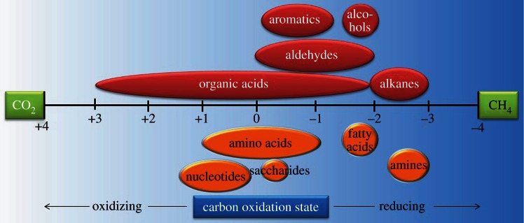
Illustration of the range of oxidation states of carbon in common biomolecules and other organic compounds.
Using essentially the same geochemical framework—mixing seawater with hydrothermal vent fluid—the thermodynamic potentials for abiotic organic synthesis were evaluated for present-day and the early Earth [42,43,46,123]. The modelling considered CO2/HCO3− reduction with H2 to generate low molecular weight hydrocarbons, alcohols, ketones, aldehydes, carboxylic acids and simple biomolecules. Based on results from earlier thermodynamic models of natural systems, high kinetic barriers were assumed for the formation of light alkanes (including methane), graphite and aromatic compounds, preventing their synthesis. It was shown that at strongly reducing conditions and corresponding high levels of H2, an aqueous mixture of inorganic and organic carbon is thermodynamically more favourable than a solution where all the carbon is CO2/HCO3− [46]. In other words, the synthesis of carboxylic acids and other low molecular weight organic compounds contributes to the Gibbs energy minimization of the overall system. The specifics of which organic compounds are energetically most likely to form and how much of the total carbon would be organic if equilibrium levels are approached, depend on the temperature, pressure and chemical composition of the system. Key controlling factors are the mineralogy of the host rock and the concentration of H2 in equilibrium with that mineralogy [24,46,116]. At equilibrium, assuming an initial oxygen fugacity (_f_O2) in the vent fluid set by the pyrite–pyrrhotite–magnetite (PPM) mineral assemblage [124,125], up to approximately 5 per cent of the total carbon would reside in simple organic compounds [46]. The most favourable conditions for thermodynamically stable organic compounds would be at approximately 100–150°C, with acetic acid/acetate dominating the distribution of organic species.
Amino acid synthesis can also be exergonic in hydrothermal systems if the appropriate reaction pathways are open. Modelling demonstrated that at 100°C and 250 bar in a mechanical mixture of seawater and vent fluid (again, based on EPR 21°N), the synthesis of 11 of the 20 amino acids from CO2 and inorganic N and S sources is exergonic [42]. It was further shown that the sum synthesis of all the requisite amino acids for thermophilic proteins (i.e. the primary structure) yielded, rather than consumed, chemical energy—up to 8 kJ mol−1 protein. Furthermore, the formation of amino acids and other organic compounds may result in surplus energy that can perhaps be shunted to the intracellular pathways for making proteins, lipids, nucleic acids and other biopolymers. At a minimum, the favourable energetics in hydrothermal systems may significantly reduce the energetic costs of biomass synthesis.
The discovery and geochemical analysis of a growing number of deep-sea hydrothermal systems spurred thermodynamic modelling to generate an ever more comprehensive picture of abiotic organic synthesis. More than 150 active submarine vents are now known from diverse tectonic settings along the ca 60 000 km-long ocean ridges and in back-arc basins [126]. Most of these systems are insufficiently characterized to permit robust energy modelling, but seven hydrothermal systems were recently investigated for their potential in abiotic organic synthesis [43]. The vent fluids at Rainbow and TAG (Mid-Atlantic Ridge), Kairei (Central Indian Ridge), Endeavor (Juan de Fuca Ridge), 9°N (East Pacific Rise), and the basins at Guaymas (Gulf of California) and Lau (southwest Pacific) are hosted in ultramafic, basalt or andesite rock, and discharging fluids range broadly in pH (2–6) and levels of dissolved hydrogen (0.37–16 mM), total sulfide (1.2–59.8 mM), ammonia (0.01–15.6 mM) and methane (0.01–63.4 mM), among other parameters.
These large differences in hydrothermal fluid compositions translate to large differences in Gibbs energies of organic synthesis reactions. The thermodynamics were consistently most favourable at the peridotite-hosted Rainbow site and the basalt-hosted Guaymas and Kairei sites—those where vent fluids have the highest H2 concentrations. In fact, the formation from CO2 of ethane, ethene, ethanol, acetaldehyde, several carboxylic acids and even some amino acids is generally exergonic at Rainbow, Guaymas and Kairei over a wide temperature range, approximately from 10°C to 200°C. At TAG, Lau Basin and Endeavor, where H2 concentrations are relatively low (0.37–0.62 mM), organic synthesis is endergonic (Δ _G_r > 0) for most reactions and temperature ranges investigated.
(i). Early Earth scenarios
The examples reviewed above considered present-day hydrothermal systems, but analogous modelling studies for the early Earth revealed even more favourable thermodynamic conditions for abiotic organic synthesis. Clearly, it is difficult to tightly constrain the composition of fluids in these cases, but reasonable assumptions can be made, especially for temperature, pH, major element chemistry and redox states of seawater and vent fluids on the early Earth. The ocean chemistry of Hadean Earth is often modelled after modern seawater, but with little, if any, dissolved oxygen. Current views on the chemistry of the Hadean atmosphere also help constrain the composition of Hadean seawater. Despite some vocal opposition [127,128], it is widely accepted that the atmosphere on the early Earth was predominantly CO2 and N2, with traces of H2, CO, CH4, NH3, H2O and reduced sulfurous gases, but essentially no free O2 [129–134]. The high CO2, in particular, would have caused warm global ocean temperatures and moderately acid pH. Because deep-sea hydrothermal fluid compositions are tightly controlled by fluid–rock interactions, and the geologic record shows that volcanic rocks from the early Earth had essentially the same bulk composition as those erupting today, the corresponding hydrothermal fluids would likely have had much the same range of compositions that we observe today.
Shock & Schulte [46] considered a range of redox states in their modelling of organic synthesis in the early Earth hydrothermal systems. They showed that a combination of inorganic and organic compounds is thermodynamically more favourable than a system with only inorganic carbon. As in the present-day example mentioned earlier, carboxylic acids dominate, but they peak at different temperatures (50–200°C), depending on the initial _f_O2 of the model hydrothermal fluid. It was calculated that carboxylic acids could account for up to approximately 45 per cent of the total carbon if the early Earth hydrothermal fluid is initially in redox equilibrium with the PPM mineral assemblage. This number reaches more than 90 per cent with hydrothermal fluids initially in redox equilibrium with fayalite–magnetite–quartz (FMQ). In fact, 100 per cent of the total carbon could be tied up in a combination of various simple aqueous organic compounds, if the initial redox state is reducing enough.
The oxidation states of submarine hydrothermal vent fluids on the early Earth likely would have varied considerably from those in present-day systems hosted in mid-ocean ridge basalt. The calculated redistribution of carbon into organic compounds, which is largely controlled by the oxidation state of the hydrothermal fluid, is illustrated in figure 2 for the early Earth. Calculations depicted in this figure, recasting results from Shock & Schulte [46], reveal the dependence of abiotic organic synthesis on the oxidation state of the fluid, as tracked by the redox parameter ƒO2. All of the results shown are for 100°C, which is reached by mixing hot vent fluids (initially at 350°C) with cold seawater (at 2°C). By combining results from models where the oxidation state of the vent fluids varies from those set at the high end by the PPM mineral assemblage to one ƒO2 unit below the oxidation state set by the FMQ mineral assemblage at the low end, it is possible to track the effects of redox variations in 100°C mixtures. It can be seen that CO2/HCO3− are dominant at the more oxidized conditions towards the right-hand side figure 2a, but that they are replaced in metastable equilibrium states by organic acids, alcohols, ketones and alkenes as the fluid mixtures become more reduced. This trend is consistent with a shift to higher H : C ratios and lower average oxidation states of carbon in the organic compounds. This shift is reflected in figure 2b that shows the distribution of the organic acids, which are summed in the single curve labelled ‘organic acids’ in figure 2a. Note that acetic acid dominates the most oxidized mixtures, followed by propanoic acid in somewhat more reduced conditions, and that the entire distribution of compounds flips over so that dodecanoic acid becomes dominant in the most reduced mixtures. The variability in ƒO2 values attainable in these examples of 100°C mixtures reflects the composition of the rocks hosting the submarine hydrothermal fluids.
Figure 2.
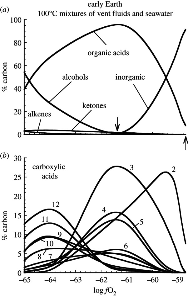
Calculated consequences for carbon speciation of attaining metastable equilibrium states at 100°C in mixtures of seawater with submarine hydrothermal vent fluids of variable initial redox state on the early Earth (derived from results presented in Shock & Schulte [46]). In (a), the upward pointing arrow indicates conditions in a 100°C mixture of seawater and 350°C vent fluid initially at PPM, and the downward pointing arrow locates conditions prevailing in a 100°C mixture of seawater and 350°C vent fluid initially at FMQ. ‘Inorganic’ refers to the sum of dissolved CO2, carbonate, bicarbonate and their complexes. In (b), numbers indicate carbon-chain length of _n_-carboxylic acids (2 = acetic acid, etc.).
The synthesis and stability of amino acid, nucleobases, ribose and deoxyribose have also been considered for the early Earth scenarios [123,135]. Redox disequilibria established from mechanical mixing of model Hadean seawater and hydrothermal fluid provides a substantial energetic drive for abiotic amino acid synthesis. As one example, thermodynamic calculations showed that at 250 bar and 100–200°C, the formation of most of the 20 protein-forming amino acids from CO2 may be exergonic [123]. Owing mostly to the major geochemical differences in seawater, the energetics are far more favourable in the Hadean Earth scenario than in the present-day analogue. It also has been suggested that the reduction of CO (rather than CO2) may have represented the first steps in the emergence of chemolithoautotrophic life [136,137]. Energy considerations show, however, that amino acid synthesis from CO, compared with that from CO2 is less favourable but still exergonic. Note that this is due in part to the two-electron difference in the carbon oxidation state between CO and CO2.
4. Organic synthesis inside the cell
In an early attempt to quantify the energetic costs of anabolism, Morowitz [138] divided cellular biomass into its constituent monomers—amino acids, nucleotides, fatty acids, saccharides and amines. This approach was later adopted and adapted to analyse energy flow for biomass synthesis in heterotrophic [139–141] and chemoautotrophic [23–25] microorganisms; the latter is reviewed here. Gibbs energies are calculated for the formation of biomonomers from inorganic starting materials (HCO3−, NH4+, HPO42−, HS−, H+ and H2). The extracellular concentrations of the reactants reflect the geochemical system of interest, and the intracellular concentrations of the biomonomers are those in the model bacterium Escherichia coli.
In several studies, the energetics were evaluated at specific oxic (actually microoxic) and anoxic conditions, as well as at conditions in present-day and the early Earth hydrothermal systems [23–25]. For the microoxic example, the _E_h was set at 0.77 eV, equivalent to an oxygen concentration of 0.1 per cent air saturation (which is less than 1 µM, a concentration that is representative for an ecosystem inhabited by microaerophiles); for the anoxic example, the _E_h was set at −0.27 eV (typical of ecosystems inhabited by methanogens and other facultative anaerobes). It was shown that the energy requirements for the autotrophic synthesis of all the biomass monomers are approximately 13 times greater under microoxic than anoxic conditions, approximately 18 400 J compared with approximately 1400 J g–1 of dry cellular biomass. When the N and S sources were NO3− and SO42− (instead of NH4+ and HS−), the energetic cost under microoxic conditions is higher still, approximately 21 600 J g−1 cells or 15 times that under anoxic conditions. This is consistent with the previously recognized higher biomass yield per unit energy in anaerobic autotrophs compared with their aerobic counterparts [142].
The energetics of biomass synthesis were also calculated in 12 deep-sea hydrothermal systems. In computer models, seawater was mixed with vent fluids in basalt (Edmond, Endeavor, EPR 21°N, Lucky Strike, TAG, Menez Gwen), peridotite (Rainbow, Logatchev, Lost City), felsic rock (Brothers, Mariner) and a troctolite–basalt hybrid (Kairei). The key geochemical parameters varied widely: pH (2.7–9), H2 (0.04–16 millimolal, m_m_), H2S (0.1–9.7 m_m_), NH4+ (0.1–503 µm) and CH4 (0.007–2.5 m_m_), among others. Consequently, the energetics of biomonomer synthesis ranged demonstrably among the different systems. Predominantly because of the high H2 levels, the formation of biomass yielded the most energy in the peridotite and troctolite–basalt hybrid systems, up to approximately 900 J g–1 dry cell mass. As noted [24], this energy yield may lessen the overall ATP requirement in growing cells, or allow ‘surplus’ ATP to be diverted to drive other, endergonic biomass synthesis reactions. In the basalt-hosted and felsic rock-hosted systems, the energetics were far less favourable even at the optimum conditions considered, with values ranging from −400 to +275 J g–1 dry cell mass.
The effect of temperature on biomass synthesis energetics was also investigated. Note that in the modelling, temperature is coupled to fluid chemistry; both are direct functions of mechanical mixing of high-temperature hydrothermal fluid of one composition with low-temperature seawater of another. It was shown that the Gibbs energies for the formation of total cell biomass as a function of temperature and seawater : hydrothermal fluid (SW : HF) mixing ratio minimize between approximately 10°C and 50°C and a SW : HF ratio of approximately 50–5 (figure 3). In seven of the 12 systems investigated (Rainbow, Logatchev, Kairei, Lost City, Endeavor, EPR 21°N, Lucky Strike), this minimum is at Δ _G_r < 0, indicating that the synthesis of cellular biomonomers is exergonic at these conditions. It should be emphasized that these calculations consider only the net energetics of reaction from inorganic compounds to biomonomers; other possible energy costs are not included so that the total anabolic process may well have a positive Gibbs energy. It should also be noted that the energetics differed demonstrably among the different biomolecule families (data not shown). Amino acid and fatty acid synthesis reactions were generally the most favourable and exergonic. The formation of amines, saccharides (both with _Δ_ _G_r ≈ 0 J g−1 dry cell mass) and nucleotides (_Δ_ _G_r > 0) is energetically much less favourable. In fact, nucleotide synthesis was endergonic in each system and at all conditions considered, perhaps reflecting the structural complexity (e.g. double-bonded carbon–nitrogen rings) and the relatively high carbon redox state (figure 1) of these compounds.
Figure 3.
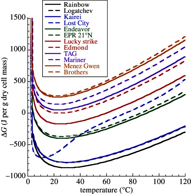
Gibbs energies (in joule per gram dry cell mass) of anabolic reactions that represent the sum total for cell biomass as a function of temperature in 12 deep-sea hydrothermal systems.
(a). From biomonomers to biopolymers
Sections 2 and 3 summarize the substantial progress that has been made in determining how chemical and physical variables affect the formation energetics of organic compounds and relatively simple biomolecules. However, microorganisms are largely composed of biomacromolecules, such as RNA, DNA, proteins, lipids and polysaccharides—these are polymeric versions of the monomers discussed earlier. Owing to the scarcity of thermodynamic data, the energetics of biomacromolecule polymerization have not received the same level of attention as their constituent monomers. Recent advances in theoretical biogeochemistry have narrowed this gap, however, and these advances are used here to compute the energetics of amino acid polymerization into proteins.
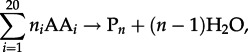
As with the condensation of nucleotides to nucleic acids and monosaccharides to polysaccharides, the polymerization of amino acids into polypeptides is a dehydration reaction that can be written as
 |
4.1 |
|---|
where AA_i_ represents any of the 20 protein-forming amino acids and P_n_ denotes a (poly)peptide consisting of n amino acid residues. The Gibbs energy of amino acid polymerization, Δ _G_1, similar to that of any other chemical reaction, is a function of temperature, pressure and composition, and it can be quantified using
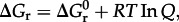 |
4.2 |
|---|
where  stands for the standard state Gibbs energy of reaction, R and T refer to the gas constant and temperature (in kelvin), respectively, and Q denotes the reaction quotient, which is defined later. Values of Δ _G_1 can be estimated at a given temperature and pressure using recently developed group contribution approaches [59,74].
The group contribution algorithm used to calculate values of  can be represented as
 |
4.3 |
|---|
where  and
and  refer to standard state Gibbs energies of formation of the protein backbone and amino acid backbone groups, respectively, which have been determined in the aqueous [61,74] and crystalline states [77]. Values of
  are shown in figure 4 from 0°C to 150°C at 500 bar (50 MPa) and at pressures corresponding to the liquid–vapour saturation pressure for water, PSAT. It can be seen in figure 4 that at both pressures,
  of amino acid polymerization increases with increasing temperature, reaching maxima at approximately 120–150°C; with a further increase in temperature,
  decreases (data not shown). It is worth noting that the pressure effect (independently of temperature) accounts for only approximately 0.5 kJ per mole of peptide bond formed, and the temperature effect from 0°C to 150°C (independently of pressure) accounts for up to 1.5 kJ per mole of peptide bond. It should also be pointed out that the polymerization energetics for these calculations are taken to be independent of the amino acid identity. This may be an oversimplification [74,77], but too few data are available in the literature to fully represent this process for all of the 20 common amino acids.
Figure 4.
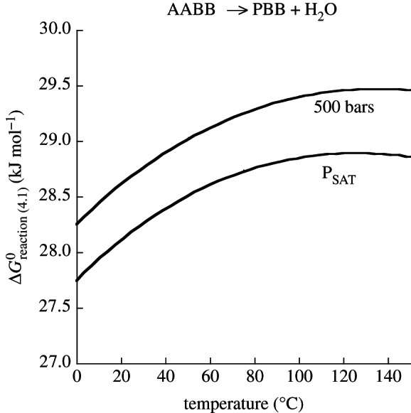
Standard state Gibbs energy of polymerizing a mole of amino acids at saturation pressure, PSAT, and at 500 bar from 0°C to 150°C.
It cannot be overemphasized that the values in figure 4 refer only to standard state conditions. In order to take into account the effects of intracellular amino acid and peptide concentrations on the Gibbs energy of polymerization, values of Q in equation (4.2) must be calculated. This can be done with
 |
4.4 |
|---|
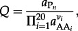
where  refers to the activity of the polypeptide of interest,
  designates the activity of the _i_th amino acid and _νi indicates the stoichiometric coefficient of the _i_th amino acid. Activity is related to concentration, C, through individual activity coefficients, _γ, consistent with
 |
4.5 |
|---|
The curves in figure 5 illustrate the effect of concentration on the energetics of polypeptide polymerization as a function of temperature for the formation of a hypothetical protein consisting of the median number of amino acid residues (278) in E. coli protein (table 1). Values of Δ _G_r were calculated with equations (4.2)–(4.4) for several total amino acid concentrations from 0.01 to 100 mM, including the average concentration of a given amino acid in E. coli cytosol, 6.5 mM (table 2). The concentration of the hypothetical E. coli peptide (P278; table 2) was 8.7 µM, and values of activity coefficients (_γ) for all aqueous species were taken to be unity. Not surprisingly, more energy is needed to polymerize a mole of this E. coli protein for lower amino acid concentrations than for higher values (figure 5). In fact, for every order of magnitude increase in amino acid concentration, there is a corresponding decrease of about 1.5 MJ required to polymerize a mole of this protein. Additionally, the effect of temperature on the energetics of protein formation is strongest at the lowest concentration, increasing from approximately 15 MJ (mol protein)−1 at 0°C to approximately 19 MJ (mol protein)−1 at 150°C.
Figure 5.
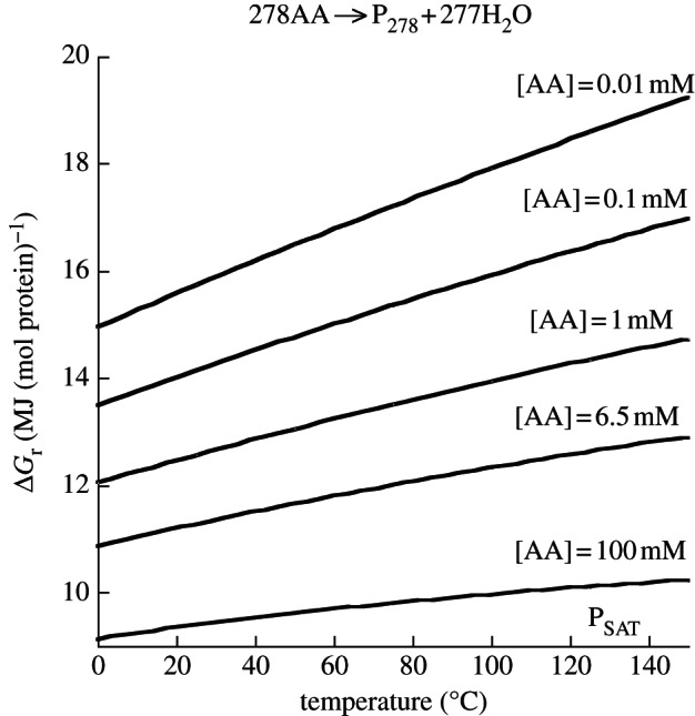
Gibbs energy required to polymerize a mole of protein consisting of the median number of amino acid residues in E. coli protein (278 AA residues) using the average concentration of protein in E. coli cytosol (8.7 µM) and various amino acid concentrations at saturation pressure from 0°C to 150°C.
Table 1.
Literature data required for peptide polymerization calculations.
| property | value | reference |
|---|---|---|
| dry mass of E. coli cell | 2.8 × 10⁻¹³ g | [143] |
| AA mass in 1 g of dry E. coli cells | 641.8 mg | calculated using data from [144]a |
| mass of free amino acids in E. coli cytosol | 41 mg | calculated using data from [145]b |
| volume of an E. coli cell | 1 µm3 | [146] |
| percentage of E. coli volume regarded as aqueous | 70% | [144] |
| mean number of AAs per protein in E. coli | 278 | [147] |
| mean number of copies of each protein in E. coli cytoplasm | 3648 | [148] |
| Gibbs energy required for de novo synthesis of all AAs in 1 g of dry E. coli cells under aerobic conditions | 11.4 kJ g–1 cell | [25] |
| Gibbs energy required for de novo synthesis of all the AAs in 1 g of dry E. coli cells under typical anaerobic conditions | 0.69 kJ g–1 cell | [25] |
Table 2.
Calculated properties of amino acids and peptides.
| derived property and source | value |
|---|---|
| mean MW of 20 common AAs | 136.90 g mol−1 |
| mean MW of the AAs found in E. coli: (% abundance) × (MW), where % abundance is from (mol AA/dry g) × (MW) × (100/total g AA per dry gram E. coli) | 133.37 g mol−1 |
| MW of average AA in a peptide: (mean AA MW) – (MW H2O) | 118.89 g mol−1 |
| MW of average AA in E. coli peptide: (weighted mean AA MW) – (MW H2O) | 115.35 g mol−1 |
| mass of protein in E. coli: (E. coli dry mass) × (% mass protein), where 55% is proteina | 1.5 × 10⁻¹³ g |
| mass of mean protein in E. coli: (avg. MW residue) × (mean E. coli polypep. length) | 32067 g mol−1 |
| mean mass of an AA in a peptide in E. coli: (weighted mean AA MW)/(_N_A) | 1.92 × 10⁻²² g |
| number of dry E. coli in a gram: 1/(dry mass of E. coli cell) | 3.6 × 10¹² |
| mass of average weighted AA residue in E. coli: (MW mean weighted AA residue)/(_N_A) | 1.915 × 10⁻²² g |
| number of AAs in proteins in E. coli: (dry mass E. coli protein)/(mass of average AA residue in E. coli in a protein) | 7.83 × 10⁸ |
| number of proteins in E. coli: (number of AAs in proteins in E. coli)/(mean number AA per protein in E. coli) | 2.82 × 10⁶ |
| concentration of average protein inside an E. coli: ((mean number of protein copies in E. coli cytoplasm)/(_N_A)) × (volume of aqueous portion of E. coli) | 8.7 × 10⁻⁶ M |
| average concentration of 17 free AA in E. coli cytosolb | 6.5 mM |
| number of polymerizations required to make all the protein in E. coli: (number of AA in proteins) – (number of proteins) | 7.80 × 10⁸ |
| number of polymerizations required to make all the peptide bonds in a dry gram of E. coli: (AA in E. coli peptides per cell) × (number dry E. coli in a gram) | 2.82 × 10²¹ |
| Gibbs energy per peptide bond formed at 25°C and 1 bar for [AA] = 6.5 mM and [P278] = 8.7 µM (see text) | 6.76 × 10⁻²⁰ J |
| Gibbs energy at 25°C and 1 bar required to make all the peptide bonds in a dry gram of E. coli for [AA] = 6.5 mM and [P278] = 8.7 µM: (Δ _G_r° per bond) × (number of peptide bonds per dry gram) | 0.191 kJ (g cell)−1 |
In a similar set of calculations, the Gibbs energies of polymerizing proteins of different lengths were also evaluated (figure 6). Here, the curves represent the energy required to polymerize a mole of median-length protein for three organisms, Pyrobaculum aerophilum, Bifidobacterium longum and Homo sapiens. The first two organisms have, respectively, the shortest and longest median protein lengths of the 83 prokaryotes given in Brocchieri & Karlin [147]; Homo sapiens was included because it is the only species that can read this. It is noteworthy that over the temperature range considered here (0–150°C), the median protein in B. longum requires over 50 per cent more energy to polymerize than the median protein in P. aerophilum. The average concentrations of amino acids and polypeptides in E. coli were used along with equations (4.2)–(4.4) to generate the curves in figure 6. Again, activity coefficients were taken to be unity.
Figure 6.
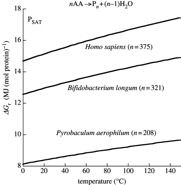
Gibbs energy of polymerizing a mole of protein of median amino acid residue length in the indicated organisms for concentrations of amino acids and protein equal to 6.5 mM and 8.7 µM, respectively, at saturation pressure from 0°C to 150°C.
To put these numbers into perspective, to make all the peptide bonds in 1 g of dry E. coli, the Gibbs energy is 0.191 kJ at 25°C, 1 bar, [AA] = 6.5 mM and [P278] = 8.7 µM (table 2), while Δ _G_r for the de novo synthesis of all the amino acids in 1 g of dry E. coli was estimated at 11.4 kJ (dry gram)−1 and 0.69 (dry gram)−1 under microoxic and anoxic conditions, respectively [25]. That is, the energy required to form all the peptide bonds in a given mass of E. coli cells in an anoxic environment is nearly 28 per cent of the energy required to synthesize all the amino acids in those proteins from inorganic constituents, such as HCO3−, NH4+ and HS−. Because the energy required to make these amino acids under microoxic conditions is more than an order of magnitude larger than that under anoxic conditions, the energy of polymerization in this instance is a rather trivial component of the total energy required to make proteins from inorganic precursors. This may seem at odds with the commonly held notion that polymerization of amino acids into peptides requires substantially more ATP than the de novo synthesis of amino acids [149]. Note, however, that the results in the current study compare the total energy required to synthesize amino acids from inorganic precursors to the subsequent polymerization of those amino acids. That is, the reactions describing the intracellular conversion of CO2 (and other reactants) into amino acids are commonly endergonic, requiring reducing power (e.g. NADPH) that is, in turn, generated from the oxidation of electron donors found in the environment. The energy associated with this transfer of electrons is accounted for in the present communication, but not in the ATP budget for microbial growth given by Stouthamer [149].
Up to this point, the energetics of amino acid synthesis have been reviewed and a procedure for calculating the energetics of amino acid polymerization into polypeptides has been demonstrated. However, in order to quantify the energetics of forming many biomacromolecules, one also must account for the energy associated with folding macromolecules into functional forms. For instance, most proteins must assume a particular three-dimensional conformation in order to perform their various structural and enzymatic roles. Below, we combine calorimetric data and the information in tables 1 and 2 to estimate the energy associated with protein folding in E. coli.
Based on compiled calorimetric data [150], the average standard state Gibbs energy of folding, based on 11 polypeptides at 25°C and 1 bar, is −0.34 kJ (mol amino acid residue)−1, with a standard deviation of −0.097 kJ (mol amino acid residue)−1. For a protein of 278 amino acid residues (the mean length in E. coli), this corresponds to −94 kJ (mol protein)−1. Using the law of mass action,
 |
4.6 |
|---|
and
 |
4.7 |
|---|
this corresponds to an equilibrium activity ratio of folded (_a_f) to unfolded proteins (_a_u) equal to 2.94 × 10¹⁶ (activity coefficients were taken to be unity). Given the aqueous volume in an E. coli cell (table 1), the concentration of a newly synthesized, yet unfolded, protein in E. coli is 2.37 × 10⁻⁹ mol l−1. Taking into account that the average concentration of the median protein in E. coli is 8.7 × 10⁻⁶ mol l−1, the Gibbs energy of folding a mole of the mean protein in E. coli is −74 kJ (mol protein)−1 ±21 kJ (using standard deviation data calculated from data in Privalov & Gill [150]) where Q = _a_f/_a_u = 3670. This is an exergonic process; hence, protein folding should be spontaneous at 25°C. As a side note, using data from Privalov & Gill [150], the standard state Gibbs energy of protein folding at 110°C and 1 bar for an E. coli protein of mean length is +278 kJ (mol protein)−1. That is, this hypothetical protein is not predicted to be folded under these conditions.
5. Conclusions
Those who use thermodynamics to evaluate the potential of organic/biomolecule synthesis in natural systems are often confronted with criticism along the lines of: (i) laboratory experiments do not support the predictions; (ii) field evidence does not support the predictions; and (ii) in biology, it is more about kinetics than thermodynamics. Let us be clear, the thermodynamic approach reviewed here informs on what is and is not energetically possible. It relies on the most accurate and internally consistent thermodynamic properties at the appropriate temperatures and pressures, as well as on detailed compositional data for the environment of interest. It serves as a framework within which to interpret experimental data and field evidence, but also to design better experiments and analyse for a wider array of compounds. The thermodynamic approach does not, however, map out what reactions will happen or what compounds will be synthesized in nature. There are certainly kinetic inhibitions to many organic reactions in hydrothermal systems, but there is also abundant evidence that some organic reactions equilibrate rapidly [151–155]. In other words, reactions involving organic compounds in hydrothermal systems are under a combination of kinetic and thermodynamic controls. Kinetic rate laws can be built into these models in the future, but at present, the requisite data are sparse. For now, thermodynamic models provide a means to evaluate which compounds might be in equilibrium and which are not, and they can identify the reactions for which there is an energetic drive at the conditions of interest.
References
- 1.Martin W, Baross JA, Kelley DS, Russell MJ. 2008. Hydrothermal vents and the origin of life. Nat. Rev. Microbiol. 6, 805–814 10.1038/nrmicro1991 (doi:10.1038/nrmicro1991) [DOI] [PubMed] [Google Scholar]
- 2.Schwartzman DW, Lineweaver CH. 2004. The hyperthermophilic origin of life revisited. Biochem. Soc. Trans. 32, 168–171 10.1042/BST0320168 (doi:10.1042/BST0320168) [DOI] [PubMed] [Google Scholar]
- 3.Pace NR. 1991. Origin of life: facing up to the physical setting. Cell 65, 531–533 10.1016/0092-8674(91)90082-A (doi:10.1016/0092-8674(91)90082-A) [DOI] [PubMed] [Google Scholar]
- 4.Cody GD, Boctor NZ, Filley TR, Hazen RM, Scott JH, Sharma A, Yoder HS., Jr 2000. Primordial carbonylated iron–sulfur compounds and the synthesis of pyruvate. Science 289, 1337–1340 10.1126/science.289.5483.1337 (doi:10.1126/science.289.5483.1337) [DOI] [PubMed] [Google Scholar]
- 5.McCollom TM, Seewald JS. 2007. Abiotic synthesis of organic compounds in deep-sea hydrothermal environments. Chem. Rev. 107, 382–401 10.1021/cr0503660 (doi:10.1021/cr0503660) [DOI] [PubMed] [Google Scholar]
- 6.McCollom TM, Ritter G, Simoneit BRT. 1999. Lipid synthesis under hydrothermal conditions by Fischer–Tropsch-type reactions. Orig. Life Evol. Biosph. 29, 153–166 10.1023/A:1006592502746 (doi:10.1023/A:1006592502746) [DOI] [PubMed] [Google Scholar]
- 7.Jakschitz TAE, Rode BM. 2012. Chemical evolution from simple inorganic compounds to chiral peptides. Chem. Soc. Rev. 41, 5484–5489 10.1039/c2cs35073d (doi:10.1039/c2cs35073d) [DOI] [PubMed] [Google Scholar]
- 8.Baross JA, Hoffman SE. 1985. Submarine hydrothermal vents and associated gradient environments as sites for the origin and evolution of life. Orig. Life 15, 327–345 10.1007/BF01808177 (doi:10.1007/BF01808177) [DOI] [Google Scholar]
- 9.Amend JP, Shock EL. 2001. Energetics of overall metabolic reactions of thermophilic and hyperthermophilic Archaea and Bacteria. FEMS Microbiol. Rev. 25, 175–243 10.1111/j.1574-6976.2001.tb00576.x (doi:10.1111/j.1574-6976.2001.tb00576.x) [DOI] [PubMed] [Google Scholar]
- 10.Pace NR. 1997. A molecular view of microbial diversity and the biosphere. Science 276, 734–740 10.1126/science.276.5313.734 (doi:10.1126/science.276.5313.734) [DOI] [PubMed] [Google Scholar]
- 11.Stetter KO. 1996. Hyperthermophilic procaryotes. FEMS Microbiol. Rev. 18, 149–158 10.1111/j.1574-6976.1996.tb00233.x (doi:10.1111/j.1574-6976.1996.tb00233.x) [DOI] [Google Scholar]
- 12.Wagner ID, Wiegel J. 2008. Diversity of thermophilic anaerobes. Ann. NY Acad. Sci. 1125, 1–43 10.1196/annals.1419.029 (doi:10.1196/annals.1419.029) [DOI] [PubMed] [Google Scholar]
- 13.Stetter KO. 2006. Hyperthermophiles in the history of life. Phil. Trans. R. Soc. B 361, 1837–1842 10.1098/rstb.2006.1907 (doi:10.1098/rstb.2006.1907) [DOI] [PMC free article] [PubMed] [Google Scholar]
- 14.Huber R, Eder W, Heldwein S, Wanner G, Huber H, Rachel R, Stetter KO. 1998. Thermocrinis ruber gen. nov., sp. nov., a pink-filament-forming hyperthermophilic bacterium isolated from Yellowstone National Park. Appl. Environ. Microbiol. 64, 3576–3583 [DOI] [PMC free article] [PubMed] [Google Scholar]
- 15.Huber R, Kristjansson JK, Stetter KO. 1987. Pyrobaculum gen. nov., a new genus group of neutrophilic, rod-shaped archaebacteria from continental solfataras growing optimally at 100°C. Arch. Microbiol. 149, 95–101 10.1007/BF00425072 (doi:10.1007/BF00425072) [DOI] [Google Scholar]
- 16.Huber R, Langworthy TA, König H, Thomm M, Woese CR, Sleytr UB, Stetter KO. 1986. Thermotoga maritima sp. nov. represents a new genus of unique extremely thermophilic eubacteria growing up to 90°C. Arch. Microbiol. 144, 324–333 10.1007/BF00409880 (doi:10.1007/BF00409880) [DOI] [Google Scholar]
- 17.Huber R, et al. 1992. Aquifex pyrophilus gen. nov. sp. nov., represents a novel group of marine hyperthermophilic hydrogen-oxidizing bacteria. Syst. Appl. Microbiol. 15, 340–351 10.1016/S0723-2020(11)80206-7 (doi:10.1016/S0723-2020(11)80206-7) [DOI] [Google Scholar]
- 18.Kurr M, Huber R, König H, Jannasch HW, Fricke H, Trincone A, Kristjansson JK, Stetter KO. 1991. Methanopyrus kandleri, gen. and sp. nov. represents a novel group of hyperthermophilic methanogens, growing to 110°C. Arch. Microbiol. 156, 239–247 10.1007/BF00262992 (doi:10.1007/BF00262992) [DOI] [Google Scholar]
- 19.Stetter KO. 1982. Ultrathin mycelia-forming organisms from submarine volcanic areas having an optimum growth temperature of 105°C. Nature 300, 258–260 10.1038/300258a0 (doi:10.1038/300258a0) [DOI] [Google Scholar]
- 20.Stetter KO. 1988. Archaeoglobus fulgidus gen . nov., sp. nov.: a new taxon of extremely thermophilic arachaebacteria. Syst. Appl. Microbiol. 10, 172–173 10.1016/S0723-2020(88)80032-8 (doi:10.1016/S0723-2020(88)80032-8) [DOI] [Google Scholar]
- 21.Takai K, et al. 2008. Cell proliferation at 122°C and isotopically heavy CH4 production by a hyperthermophilic methanogen under high-pressure cultivation. Proc. Natl Acad. Sci. USA 105, 10 949–10 954 10.1073/pnas.0707900105 (doi:10.1073/pnas.0707900105) [DOI] [PMC free article] [PubMed] [Google Scholar]
- 22.Cox A, Shock EL, Havig JR. 2011. The transition to microbial photosynthesis in hot spring ecosystems. Chem. Geol. 280, 344–351 10.1016/j.chemgeo.2010.11.022 (doi:10.1016/j.chemgeo.2010.11.022) [DOI] [Google Scholar]
- 23.Amend JP, McCollom TM. 2009. Energetics of biomolecule synthesis on early Earth. In Chemical evolution II: from the origins of life to modern society (eds Zaikowski L, Friedrich JM, Seidel SR.), pp. 63–94 ACS Symposium Series Washington, DC: American Chemical Society [Google Scholar]
- 24.Amend JP, McCollom TM, Hentscher M, Bach W. 2011. Catabolic and anabolic energy for chemolithoautotrophs in deep-sea hydrothermal systems hosted in different rock types. Geochim. Cosmochim. Acta 75, 5736–5748 10.1016/j.gca.2011.07.041 (doi:10.1016/j.gca.2011.07.041) [DOI] [Google Scholar]
- 25.McCollom TM, Amend JP. 2005. A thermodynamic assessment of energy requirements for biomass synthesis by chemolithoautotrophic micro-organisms in oxic and anoxic environments. Geobiology 3, 135–144 10.1111/j.1472-4669.2005.00045.x (doi:10.1111/j.1472-4669.2005.00045.x) [DOI] [Google Scholar]
- 26.Shock EL, Helgeson HC. 1990. Calculation of the thermodynamic and transport properties of aqueous species at high pressures and temperatures: standard partial molal properties of organic species. Geochim. Cosmochim. Acta 54, 915–945 10.1016/0016-7037(90)90429-O (doi:10.1016/0016-7037(90)90429-O) [DOI] [Google Scholar]
- 27.Shock EL, Helgeson HC. 1988. Calculation of the thermodynamic and transport properties of aqueous species at high pressures and temperatures: correlation algorithms for ionic species and equation of state predictions to 5 kb and 1000°C. Geochim. Cosmochim. Acta 52, 2009–2036 10.1016/0016-7037(88)90181-0 (doi:10.1016/0016-7037(88)90181-0) [DOI] [Google Scholar]
- 28.Shock EL, Helgeson HC, Sverjensky DA. 1989. Calculation of the thermodynamic and transport properties of aqueous species at high pressures and temperatures: standard partial molal properties of inorganic neutral species. Geochim. Cosmochim. Acta 53, 2157–2183 10.1016/0016-7037(89)90341-4 (doi:10.1016/0016-7037(89)90341-4) [DOI] [Google Scholar]
- 29.Helgeson HC, Delany JM, Nesbitt WH, Bird DK. 1978. Summary and critique of the thermodynamic properties of rock-forming minerals. Am. J. Sci. 278A, 1–229 [Google Scholar]
- 30.Haas JR, Shock EL, Sassani DC. 1995. Rare earth elements in hydrothermal systems: estimates of standard partial molal thermodynamic properties of aqueous complexes of the REE at high pressures and temperatures. Geochim. Cosmochim. Acta 59, 4329–4350 10.1016/0016-7037(95)00314-P (doi:10.1016/0016-7037(95)00314-P) [DOI] [Google Scholar]
- 31.Shock EL, Sassani DC, Willis M, Sverjensky DA. 1997. Inorganic species in geologic fluids: correlations among standard molal thermodynamic properties of aqueous ions and hydroxide complexes. Geochim. Cosmochim. Acta 61, 907–950 10.1016/S0016-7037(96)00339-0 (doi:10.1016/S0016-7037(96)00339-0) [DOI] [PubMed] [Google Scholar]
- 32.Shock EL, Sassani DC, Betz H. 1997. Uranium in geologic fluids: estimates of standard partial molal properties, oxidation potentials, and hydrolysis constants at high temperatures and pressures. Geochim. Cosmochim. Acta 61, 4245–4266 10.1016/S0016-7037(97)00240-8 (doi:10.1016/S0016-7037(97)00240-8) [DOI] [Google Scholar]
- 33.Sverjensky DA, Shock EL, Helgeson HC. 1997. Prediction of the thermodynamic and transport properties of aqueous metal complexes to 1000°C and 5 kb. Geochim. Cosmochim. Acta 61, 1359–1412 10.1016/S0016-7037(97)00009-4 (doi:10.1016/S0016-7037(97)00009-4) [DOI] [PubMed] [Google Scholar]
- 34.Sassani DC, Shock EL. 1998. Solubility and transport of platinum-group elements in supercritical fluids: summary and estimates of thermodynamic properties for Ru, Rh, Pd, and Pt solids, aqueous ions and aqueous complexes. Geochim. Cosmochim. Acta 62, 2643–2671 10.1016/S0016-7037(98)00049-0 (doi:10.1016/S0016-7037(98)00049-0) [DOI] [Google Scholar]
- 35.Murphy WM, Shock EL. 1999. Environmental aqueous geochemistry of actinides. Rev Mineral 38, 221–253 [Google Scholar]
- 36.Shock EL, Oelkers EH, Johnson JW, Sverjensky DA, Helgeson HC. 1992. Calculation of the thermodynamic properties of aqueous species at high pressures and temperatures: effective electrostatic radii, dissociation constants and standard partial molal properties to 1000 °C and 5 kbar. J. Chem. Soc. Faraday Trans. 88, 803–826 10.1039/ft9928800803 (doi:10.1039/ft9928800803) [DOI] [Google Scholar]
- 37.Tanger JC, Helgeson HC. 1988. Calculation of the thermodynamic and transport properties of aqueous species at high pressures and temperatures: revised equations of state for the standard partial molal properties of ions and electrolytes. Am. J. Sci. 288, 19–98 10.2475/ajs.288.1.19 (doi:10.2475/ajs.288.1.19) [DOI] [Google Scholar]
- 38.Shock EL. 1988. Organic acid metastability in sedimentary basins. Geology 16, 886–890 10.1130/0091-7613(1988)016<0886:OAMISB>2.3.CO;2 (doi:10.1130/0091-7613(1988)016<0886:OAMISB>2.3.CO;2) [DOI] [Google Scholar]
- 39.Shock EL. 1989. Corrections to ‘Organic acid metastability in sedimentary basins’. Geology 17, 572–573 10.1130/0091-7613(1989)017<0572:CTOAMI>2.3.CO;2 (doi:10.1130/0091-7613(1989)017<0572:CTOAMI>2.3.CO;2) [DOI] [Google Scholar]
- 40.Shock EL. 1994. Application of thermodynamic calculations to geochemical processes involving organic acids. In The role of organic acids in geological processes (eds Lewan M, Pittman E.), pp. 270–318 Berlin, Germany: Springer [Google Scholar]
- 41.Helgeson HC, Knox AM, Owens CE, Shock EL. 1993. Petroleum, oil field waters, and authigenic mineral assemblages: are they in metastable equilibrium in hydrocarbon reservoirs? Geochim. Cosmochim. Acta 57, 3295–3339 10.1016/0016-7037(93)90541-4 (doi:10.1016/0016-7037(93)90541-4) [DOI] [Google Scholar]
- 42.Amend JP, Shock EL. 1998. Energetics of amino acid synthesis in hydrothermal ecosystems. Science 281, 1659–1662 10.1126/science.281.5383.1659 (doi:10.1126/science.281.5383.1659) [DOI] [PubMed] [Google Scholar]
- 43.Shock E, Canovas P. 2010. The potential for abiotic organic synthesis and biosynthesis at seafloor hydrothermal systems. Geofluids 10, 161–192 10.1111/j.1468-8123.2010.00277.x (doi:10.1111/j.1468-8123.2010.00277.x) [DOI] [Google Scholar]
- 44.Shock EL. 1990. Geochemical constraints on the origin of organic compounds in hydrothermal systems. Orig. Life Evol. Biosph. 20, 331–367 10.1007/BF01808115 (doi:10.1007/BF01808115) [DOI] [PubMed] [Google Scholar]
- 45.Shock EL. 1992. Chemical environments of submarine hydrothermal systems. Orig. Life Evol. Biosph. 22, 67–107 10.1007/BF01808019 (doi:10.1007/BF01808019) [DOI] [PubMed] [Google Scholar]
- 46.Shock EL, Schulte MD. 1998. Organic synthesis during fluid mixing in hydrothermal systems. J. Geophys. Res. 103, 28 513–28 527 10.1029/98JE02142 (doi:10.1029/98JE02142) [DOI] [Google Scholar]
- 47.Schulte MD, Shock EL. 1993. Aldehydes in hydrothermal solution: standard partial molal thermodynamic properties and relative stabilities at high temperatures and pressures. Geochim. Cosmochim. Acta 57, 3835–3846 10.1016/0016-7037(93)90337-V (doi:10.1016/0016-7037(93)90337-V) [DOI] [PubMed] [Google Scholar]
- 48.Shock EL. 1992. Stability of peptides in high-temperature aqueous solutions. Geochim. Cosmochim. Acta 56, 3481–3491 10.1016/0016-7037(92)90392-V (doi:10.1016/0016-7037(92)90392-V) [DOI] [Google Scholar]
- 49.Dale JD, Shock EL, Macleod G, Aplin AC, Larter SR. 1997. Standard partial molal properties of aqueous alkylphenols at high pressures and temperatures. Geochim. Cosmochim. Acta 61, 4017–4024 10.1016/S0016-7037(97)00212-3 (doi:10.1016/S0016-7037(97)00212-3) [DOI] [Google Scholar]
- 50.Shock EL. 1995. Organic acids in hydrothermal solutions: standard molal thermodynamic properties of carboxylic acids, and estimates of dissociation constants at high temperatures and pressures. Am. J. Sci. 295, 496–580 10.2475/ajs.295.5.496 (doi:10.2475/ajs.295.5.496) [DOI] [PubMed] [Google Scholar]
- 51.Prapaipong P, Shock EL, Koretsky CM. 1999. Metal-organic complexes in geochemical processes: temperature dependence of the standard thermodynamic properties of aqueous complexes between metal cations and dicarboxylate ligands. Geochim. Cosmochim. Acta 63, 2547–2577 10.1016/S0016-7037(99)00146-5 (doi:10.1016/S0016-7037(99)00146-5) [DOI] [Google Scholar]
- 52.Shock EL, Koretsky CM. 1993. Metal-organic complexes in geochemical processes—calculation of standard partial molal thermodynamic properties of aqueous acetate complexes at high pressures and temperatures. Geochim. Cosmochim. Acta 57, 4899–4922 10.1016/0016-7037(93)90128-J (doi:10.1016/0016-7037(93)90128-J) [DOI] [Google Scholar]
- 53.Shock EL, Koretsky CM. 1995. Metal-organic complexes in geochemical processes: estimation of standard partial molal thermodynamic properties of aqueous complexes between metal cations and monovalent organic acid ligands at high pressures and temperatures. Geochim. Cosmochim. Acta 59, 1497–1532 10.1016/0016-7037(95)00058-8 (doi:10.1016/0016-7037(95)00058-8) [DOI] [Google Scholar]
- 54.Haas JR, Shock EL. 1999. Halocarbons in the environment: estimates of thermodynamic properties for aqueous chloroethylene species and their stabilities in natural settings. Geochim. Cosmochim. Acta 63, 3429–3441 10.1016/S0016-7037(99)00276-8 (doi:10.1016/S0016-7037(99)00276-8) [DOI] [Google Scholar]
- 55.Amend JP, Plyasunov AV. 2001. Carbohydrates in thermophile metabolism: calculation of the standard molal thermodynamic properties of aqueous pentoses and hexoses at elevated temperatures and pressures. Geochim. Cosmochim. Acta 65, 3901–3917 10.1016/S0016-7037(01)00707-4 (doi:10.1016/S0016-7037(01)00707-4) [DOI] [Google Scholar]
- 56.Schulte MD, Rogers KL. 2004. Thiols in hydrothermal solution: standard partial molal properties and their role in the organic geochemistry of hydrothermal environments. Geochim. Cosmochim. Acta 68, 1087–1097 10.1016/j.gca.2003.06.001 (doi:10.1016/j.gca.2003.06.001) [DOI] [Google Scholar]
- 57.Schulte M. 2010. Organic sulfides in hydrothermal solution: standard partial molal properties and role in organic geochemistry of hydrothermal environments. Aquat. Geochem. 16, 621–637 10.1007/s10498-010-9102-3 (doi:10.1007/s10498-010-9102-3) [DOI] [Google Scholar]
- 58.Plyasunov AV, Shock EL. 2001. A correlation strategy for determining the parameters of the revised-HKF model for aqueous nonelectrolytes. Geochim. Cosmochim. Acta 65, 3879–3900 10.1016/S0016-7037(01)00678-0 (doi:10.1016/S0016-7037(01)00678-0) [DOI] [Google Scholar]
- 59.Amend JP, Helgeson HC. 1997. Group additivity equations of state for calculating the standard molal thermodynamic properties of aqueous organic molecules at elevated temperatures and pressures. Geochim. Cosmochim. Acta 61, 11–46 10.1016/S0016-7037(96)00306-7 (doi:10.1016/S0016-7037(96)00306-7) [DOI] [Google Scholar]
- 60.Amend JP, Helgeson HC. 1997. Calculation of the standard molal thermodynamic properties of aqueous biomolecules at elevated temperatures and pressures. I. L-α-amino acids. J. Chem. Soc. Faraday Trans. 93, 1927–1941 10.1039/A608126F (doi:10.1039/A608126F) [DOI] [PubMed] [Google Scholar]
- 61.Amend JP, Helgeson HC. 2000. Calculation of the standard molal thermodynamic properties of aqueous biomolecules at elevated temperatures and pressures. II. Unfolded proteins. Biophys. Chem. 84, 105–136 10.1016/S0301-4622(00)00116-2 (doi:10.1016/S0301-4622(00)00116-2) [DOI] [PubMed] [Google Scholar]
- 62.Helgeson HC, Owens CE, Knox AM, Richard L. 1998. Calculation of the standard molal thermodynamic properties of crystalline, liquid, and gas organic molecules at high temperatures and pressures. Geochim. Cosmochim. Acta 62, 985–1081 10.1016/S0016-7037(97)00219-6 (doi:10.1016/S0016-7037(97)00219-6) [DOI] [Google Scholar]
- 63.Amend JP, Helgeson HC. 1997. Solubilities of the common L-α-amino acids as a function of temperature and solution pH. Pure Appl. Chem. 69, 935–942 10.1351/pac199769050935 (doi:10.1351/pac199769050935) [DOI] [Google Scholar]
- 64.Richard L. 2001. Calculation of the standard molal thermodynamic properties as a function of temperature and pressure of some geochemically important organic sulfur compounds. Geochim. Cosmochim. Acta 65, 3827–3877 10.1016/S0016-7037(01)00761-X (doi:10.1016/S0016-7037(01)00761-X) [DOI] [Google Scholar]
- 65.Richard L, Helgeson HC. 1998. Calculation of the thermodynamic properties at elevated temperatures and pressures of saturated and aromatic high molecular weight solid and liquid hydrocarbons in kerogen, bitumen, petroleum, and other organic matter of biogeochemical interest. Geochim. Cosmochim. Acta 62, 3591–3636 10.1016/S0016-7037(97)00345-1 (doi:10.1016/S0016-7037(97)00345-1) [DOI] [Google Scholar]
- 66.Plyasunov AV, Shock EL. 2000. Thermodynamic functions of hydration of hydrocarbons at 298.15 K and 0.1 MPa. Geochim. Cosmochim. Acta 64, 439–468 10.1016/S0016-7037(99)00330-0 (doi:10.1016/S0016-7037(99)00330-0) [DOI] [Google Scholar]
- 67.Plyasunov AV, Shock EL. 2000. Standard state Gibbs energies of hydration of hydrocarbons at elevated temperatures as evaluated from experimental phase equilibria studies. Geochim. Cosmochim. Acta 64, 2811–2833 10.1016/S0016-7037(00)00401-4 (doi:10.1016/S0016-7037(00)00401-4) [DOI] [Google Scholar]
- 68.Plyasunov AV, Shock EL. 2001. Group contribution values of the infinite dilution thermodynamic functions of hydration for aliphatic noncyclic hydrocarbons, alcohols, and ketones at 298.15 K and 0.1 MPa. J. Chem. Eng. Data 46, 1016–1019 10.1021/je0002282 (doi:10.1021/je0002282) [DOI] [Google Scholar]
- 69.Plyasunov AV, Plyasunova NV, Shock EL. 2004. Group contribution values for the thermodynamic functions of hydration of aliphatic esters at 298.15 K, 0.1 MPa. J. Chem. Eng. Data 49, 1152–1167 10.1021/je049850a (doi:10.1021/je049850a) [DOI] [Google Scholar]
- 70.Plyasunova NV, Plyasunov AV, Shock EL. 2005. Group contribution values for the thermodynamic functions of hydration at 298.15 K, 0.1 MPa. 2. Aliphatic thiols, alkyl sulfides, and polysulfides. J. Chem. Eng. Data 50, 246–253 10.1021/je0497045 (doi:10.1021/je0497045) [DOI] [Google Scholar]
- 71.Plyasunov AV, Plyasunova NV, Shock EL. 2006. Group contribution values for the thermodynamic functions of hydration at 298.15 K, 0.1 MPa. 3. Aliphatic monoethers, diethers, and polyethers. J. Chem. Eng. Data 51, 276–290 10.1021/je050390a (doi:10.1021/je050390a) [DOI] [Google Scholar]
- 72.Plyasunov AV, Plyasunova NV, Shock EL. 2006. Group contribution values for the thermodynamic functions of hydration at 298.15 K, 0.1 MPa. 4. Aliphatic nitriles and dinitriles. J. Chem. Eng Data 51, 1481–1490 10.1021/je060129+ (doi:10.1021/je060129+) [DOI] [Google Scholar]
- 73.Plyasunova NV, Plyasunov AV, Shock EL. 2004. Database of thermodynamic properties for aqueous organic compounds. Int. J. Thermophys. 25, 351–360 10.1023/B:IJOT.0000028472.63853.2d (doi:10.1023/B:IJOT.0000028472.63853.2d) [DOI] [Google Scholar]
- 74.Dick JM, LaRowe DE, Helgeson HC. 2006. Temperature, pressure, and electrochemical constraints on protein speciation: group additivity calculation of the standard molal thermodynamic properties of ionized unfolded proteins. Biogeosciences 3, 311–336 10.5194/bg-3-311-2006 (doi:10.5194/bg-3-311-2006) [DOI] [Google Scholar]
- 75.LaRowe DE, Helgeson HC. 2006. Biomolecules in hydrothermal systems: calculation of the standard molal thermodynamic properties of nucleic-acid bases, nucleosides, and nucleotides at elevated temperatures and pressures. Geochim. Cosmochim. Acta 70, 4680–4724 10.1016/j.gca.2006.04.010 (doi:10.1016/j.gca.2006.04.010) [DOI] [Google Scholar]
- 76.LaRowe DE, Helgeson HC. 2006. The energetics of metabolism in hydrothermal systems: calculation of the standard molal thermodynamic properties of magnesium-complexed adenosine nucleotides and NAD and NADP at elevated temperatures and pressures. Thermochim. Acta 448, 82–106 10.1016/j.tca.2006.06.008 (doi:10.1016/j.tca.2006.06.008) [DOI] [Google Scholar]
- 77.LaRowe DE, Dick JM. 2012. Calculation of the standard molal thermodynamic properties of crystalline peptides. Geochim. Cosmochim. Acta 80, 70–91 10.1016/j.gca.2011.11.041 (doi:10.1016/j.gca.2011.11.041) [DOI] [Google Scholar]
- 78.LaRowe DE, Van Cappellen P. 2011. Degradation of natural organic matter: a thermodynamic analysis. Geochim. Cosmochim. Acta 75, 2030–2042 10.1016/j.gca.2011.01.020 (doi:10.1016/j.gca.2011.01.020) [DOI] [Google Scholar]
- 79.LaRowe DE, Dale AW, Amend JP, Van Cappellen P. 2012. Thermodynamic limitations on microbially catalyzed reaction rates. Geochim. Cosmochim. Acta 90, 96–109 10.1016/j.gca.2012.05.011 (doi:10.1016/j.gca.2012.05.011) [DOI] [Google Scholar]
- 80.Dick JM, Shock EL. 2011. Calculation of the relative chemical stabilities of proteins as a function of temperature and redox chemistry in a hot spring. PLoS ONE 6, e22782. 10.1371/journal.pone.0022782 (doi:10.1371/journal.pone.0022782) [DOI] [PMC free article] [PubMed] [Google Scholar]
- 81.Berndt ME, Allen DE, Seyfried WEJ. 1996. Reduction of CO2 during serpentinization of olivine at 300°C and 500 bar. Geology 24, 351–354 10.1130/0091-7613(1996)024<0351:ROCDSO>2.3.CO;2 (doi:10.1130/0091-7613(1996)024<0351:ROCDSO>2.3.CO;2) [DOI] [Google Scholar]
- 82.Foustoukos DI, Seyfried WE. 2004. Hydrocarbons in hydrothermal vent fluids: the role of chromium-bearing catalysts. Science 304, 1002–1005 10.1126/science.1096033 (doi:10.1126/science.1096033) [DOI] [PubMed] [Google Scholar]
- 83.Fu Q, Lollar BS, Horita J, Lacrampe-Couloume G, Seyfried WE. 2007. Abiotic formation of hydrocarbons under hydrothermal conditions: constraints from chemical and isotope data. Geochim. Cosmochim. Acta 71, 1982–1998 10.1016/j.gca.2007.01.022 (doi:10.1016/j.gca.2007.01.022) [DOI] [Google Scholar]
- 84.Horita J, Berndt ME. 1999. Abiogenic methane formation and isotopic fractionation under hydrothermal conditions. Science 285, 1055–1057 10.1126/science.285.5430.1055 (doi:10.1126/science.285.5430.1055) [DOI] [PubMed] [Google Scholar]
- 85.McCollom TM, Seewald JS. 2001. A reassessment of the potential for reduction of dissolved CO2 to hydrocarbons during serpentinization of olivine. Geochim. Cosmochim. Acta 65, 3769–3778 10.1016/S0016-7037(01)00655-X (doi:10.1016/S0016-7037(01)00655-X) [DOI] [Google Scholar]
- 86.McCollom TM, Seewald JS. 2006. Carbon isotope composition of organic compounds produced by abiotic synthesis under hydrothermal conditions. Earth Planet Sci. Lett. 243, 74–84 10.1016/j.epsl.2006.01.027 (doi:10.1016/j.epsl.2006.01.027) [DOI] [Google Scholar]
- 87.Charlou J-L, Donval JP, Konn C, Ondreas H, Fouquet Y. 2010. High production and fluxes of H2 and CH4 and evidence of abiotic hydrocarbons synthesis by serpentinization in ultramafic-hosted hydrothermal systems on the Mid-Atlantic Ridge. In Diversity of hydrothermal systems on slow spreading ocean ridges (eds Rona PA, Devey C, Dyment J, Murton BJ.), pp. 265–296 Washington, DC: American Geophysical Union [Google Scholar]
- 88.Lang SQ, Butterfield D, Schulte M, Kelley DS, Lilley MD. 2010. Elevated concentrations of formate, acetate and dissolved organic carbon found at the Lost City hydrothermal field. Geochim. Cosmochim. Acta 74, 941–952 10.1016/j.gca.2009.10.045 (doi:10.1016/j.gca.2009.10.045) [DOI] [Google Scholar]
- 89.Proskurowski G, Lilley MD, Seewald JS, Früh-Green GL, Olson EJ, Lupton JE, Sylva SP, Kelley DS. 2008. Abiogenic hydrocarbon production at Lost City hydrothermal field. Science 319, 604–607 10.1126/science.1151194 (doi:10.1126/science.1151194) [DOI] [PubMed] [Google Scholar]
- 90.Fox SW, Windsor CR. 1970. Synthesis of amino acids by the heating of formaldehyde and ammonia. Science 170, 984–986 10.1126/science.170.3961.984 (doi:10.1126/science.170.3961.984) [DOI] [PubMed] [Google Scholar]
- 91.Hennet RJ-C, Holm NG, Engel MH. 1992. Abiotic synthesis of amino acids under hydrothermal conditions and the origin of life: a perpetual phenomenon? Naturwissenschaften 79, 361–365 10.1007/BF01140180 (doi:10.1007/BF01140180) [DOI] [PubMed] [Google Scholar]
- 92.Huber C, Wachterschauser G. 2006. _α_-Hydroxy and _α_-amino acids under possible Hadean, volcanic origin-of-life conditions. Science 314, 630–632 10.1126/science.1130895 (doi:10.1126/science.1130895) [DOI] [PubMed] [Google Scholar]
- 93.Keefe AD, Miller SL, Mcdonald G, Bada J. 1995. Investigation of the prebiotic synthesis of amino-acids and RNA bases from CO2 using FeS/H2S as a reducing agent. Proc. Natl Acad. Sci. USA 92, 11 904–11 906 10.1073/pnas.92.25.11904 (doi:10.1073/pnas.92.25.11904) [DOI] [PMC free article] [PubMed] [Google Scholar]
- 94.Lowe CU, Markham R, Rees MW. 1963. Synthesis of complex organic compounds from simple precursors—formation of amino-acids, amino-acid polymers, fatty acids and purines from ammonium cyanide. Nature 199, 219–222 10.1038/199219a0 (doi:10.1038/199219a0) [DOI] [PubMed] [Google Scholar]
- 95.Marshall WL. 1994. Hydrothermal synthesis of amino acids. Geochim. Cosmochim. Acta 58, 2099–2106 10.1016/0016-7037(94)90288-7 (doi:10.1016/0016-7037(94)90288-7) [DOI] [Google Scholar]
- 96.Oro J, Kamat SS. 1961. Amino-acid synthesis from hydrogen cyanide under possible primitive earth conditions. Nature 190, 442–444 10.1038/190442a0 (doi:10.1038/190442a0) [DOI] [PubMed] [Google Scholar]
- 97.Oro J, Kimball A, Fritz R, Master F. 1959. Amino acid synthesis from formaldehyde and hydroxylamine. Arch. Biochem. Biophys. 85, 115–130 10.1016/0003-9861(59)90455-2 (doi:10.1016/0003-9861(59)90455-2) [DOI] [PubMed] [Google Scholar]
- 98.Butlerov A. 1861. Formation synthétique d'une substance sucrée. Compt. Rend. Acad. Sci. 53, 145–147 [Google Scholar]
- 99.Breslow R. 1959. On the mechanism of the formose reaction. Tetrahedron Lett. 1, 22–26 10.1016/S0040-4039(01)99487-0 (doi:10.1016/S0040-4039(01)99487-0) [DOI] [Google Scholar]
- 100.Oro J. 1960. Synthesis of adenine from ammonium cyanide. Biochem. Biophys. Res. Commun. 2, 407–412 10.1016/0006-291X(60)90138-8 (doi:10.1016/0006-291X(60)90138-8) [DOI] [Google Scholar]
- 101.Sanchez RA, Ferris JP, Orgel LE. 1967. Studies in prebiotic synthesis 0.2. Synthesis of purine precursors and amino acids from aqueous hydrogen cyanide. J. Mol. Biol. 30, 223–253 [PubMed] [Google Scholar]
- 102.Fox SW, Harada K. 1961. Synthesis of uracil under conditions of a thermal model of prebiological chemistry. Science 133, 1923–1924 10.1126/science.133.3468.1923 (doi:10.1126/science.133.3468.1923) [DOI] [PubMed] [Google Scholar]
- 103.Sanchez RA, Ferris JP, Orgel LE. 1966. Cyanoacetylene in prebiotic synthesis. Science 154, 784–785 10.1126/science.154.3750.784 (doi:10.1126/science.154.3750.784) [DOI] [PubMed] [Google Scholar]
- 104.Saladino R, Ciambecchini U, Crestini C, Costanzo G, Negri R, Di Mauro E. 2003. One-pot TiO2-catalyzed synthesis of nucleic bases and acyclonucleosides from formamide: implications for the origin of life. Chembiochem 4, 514–521 10.1002/cbic.200300567 (doi:10.1002/cbic.200300567) [DOI] [PubMed] [Google Scholar]
- 105.Saladino R, Crestini C, Ciambecchini U, Ciciriello F, Costanzo G, Di Mauro E. 2004. Synthesis and degradation of nucleobases and nucleic acids by formamide in the presence of montmorillonites. Chembiochem 5, 1558–1566 10.1002/cbic.200400119 (doi:10.1002/cbic.200400119) [DOI] [PubMed] [Google Scholar]
- 106.Aubrey AD, Cleaves HJ, Bada JL. 2009. The role of submarine hydrothermal systems in the synthesis of amino acids. Orig. Life Evol. B 39, 91–108 10.1007/s11084-008-9153-2 (doi:10.1007/s11084-008-9153-2) [DOI] [PubMed] [Google Scholar]
- 107.Shapiro R. 1988. Prebiotic ribose synthesis: a critical analysis. Orig. Life Evol. Biosph. 18, 71–85 10.1007/BF01808782 (doi:10.1007/BF01808782) [DOI] [PubMed] [Google Scholar]
- 108.Shapiro R. 1995. The prebiotic role of adenine: a critical analysis. Orig. Life Evol. Biosph. 25, 83–98 10.1007/BF01581575 (doi:10.1007/BF01581575) [DOI] [PubMed] [Google Scholar]
- 109.Shapiro R. 1999. Prebiotic cytosine synthesis: a critical analysis and implications for the origin of life. Proc. Natl Acad. Sci. USA 96, 4396–4401 10.1073/pnas.96.8.4396 (doi:10.1073/pnas.96.8.4396) [DOI] [PMC free article] [PubMed] [Google Scholar]
- 110.Abrajano TA, Sturchio NC, Kennedy BM, Lyon GL, Muehlenbachs K, Bohlke JK. 1990. Geochemistry of reduced gas related to serpentinization of the zambales ophiolite. Philippines Appl. Geochem. 5, 625–630 10.1016/0883-2927(90)90060-I (doi:10.1016/0883-2927(90)90060-I) [DOI] [Google Scholar]
- 111.Sherwood Lollar B, Lacrampe-Couloume G, Slater GF, Ward J, Moser DP, Gihring TM, Lin L.-H., Onstott TC. 2006. Unravelling abiogenic and biogenic sources of methane in the Earth's deep subsurface. Chem. Geol. 226, 328–339 10.1016/j.chemgeo.2005.09.027 (doi:10.1016/j.chemgeo.2005.09.027) [DOI] [Google Scholar]
- 112.Sherwood Lollar B, Lacrampe-Couloume G, Voglesonger K, Onstott TC, Pratt LM, Slater GF. 2008. Isotopic signatures of CH4 and higher hydrocarbon gases from Precambrian Shield sites: a model for abiogenic polymerization of hydrocarbons. Geochim. Cosmochim. Acta 72, 4778–4795 10.1016/j.gca.2008.07.004 (doi:10.1016/j.gca.2008.07.004) [DOI] [Google Scholar]
- 113.Taran YA, Varley NR, Inguaggiato S, Cienfuegos E. 2010. Geochemistry of H2 and CH4-enriched hydrothermal fluids of Socorro Island, Revillagigedo Archipelago, Mexico. Evidence for serpentinization and abiogenic methane. Geofluids 10, 542–555 10.1111/j.1468-8123.2010.00314.x (doi:10.1111/j.1468-8123.2010.00314.x) [DOI] [Google Scholar]
- 114.Holm NG, Charlou JL. 2001. Initial indications of abiotic formation of hydrocarbons in the Rainbow ultramafic hydrothermal system. Earth Planet Sci. Lett. 191, 1–8 10.1016/S0012-821X(01)00397-1 (doi:10.1016/S0012-821X(01)00397-1) [DOI] [Google Scholar]
- 115.Konn C, Charlou JL, Donval JP, Holm NG, Dehairs F, Bouillon S. 2009. Hydrocarbons and oxidized organic compounds in hydrothermal fluids from Rainbow and Lost City ultramafic hosted vents. Chem. Geol. 258, 299–314 10.1016/j.chemgeo.2008.10.034 (doi:10.1016/j.chemgeo.2008.10.034) [DOI] [Google Scholar]
- 116.McCollom TM. 2007. Geochemical constraints on sources of metabolic energy for chemolithoautotrophy in ultramafic-hosted deep-sea hydrothermal systems. Astrobiology 7, 933–950 10.1089/ast.2006.0119 (doi:10.1089/ast.2006.0119) [DOI] [PubMed] [Google Scholar]
- 117.Cronin J, Pizzarello S, Cruikshank DP. 1988. Organic matter in carbonaceous chondrites, planetary satellites, asteroids, and comets. In Meteorites and the early Solar System (eds Kerridge JF, Mathews MS.), pp. 819–857 Tucson, AZ: University of Arizona Press [Google Scholar]
- 118.Pizzarello S. 2007. The chemistry that preceded life's origin: a study guide from meteorites. Chem. Biodivers. 4, 680–693 10.1002/cbdv.200790058 (doi:10.1002/cbdv.200790058) [DOI] [PubMed] [Google Scholar]
- 119.Pizzarello S, Shock E. 2010. The organic composition of carbonaceous meteorites: the evolutionary story ahead of biochemistry. Cold Spring Harb. Perspect. Biol. 2, a002105. 10.1101/cshperspect.a002105 (doi:10.1101/cshperspect.a002105) [DOI] [PMC free article] [PubMed] [Google Scholar]
- 120.McCollom TM, Shock EL. 1997. Geochemical constraints on chemolithoautotrophic metabolism by microorganisms in seafloor hydrothermal systems. Geochim. Cosmochim. Acta 61, 4375–4391 10.1016/S0016-7037(97)00241-X (doi:10.1016/S0016-7037(97)00241-X) [DOI] [PubMed] [Google Scholar]
- 121.Von Damm KL. 1990. Seafloor hydrothermal activity: black smoker chemistry and chimneys. Ann. Rev. Earth Planet Sci. 18, 173–204 10.1146/annurev.ea.18.050190.001133 (doi:10.1146/annurev.ea.18.050190.001133) [DOI] [Google Scholar]
- 122.Von Damm KL, Edmond JM, Grant B, Measures CI, Walden B, Weiss RF. 1985. Chemistry of submarine hydrothermal solutions at 21°N, East Pacific Rise. Geochim. Cosmochim. Acta 49, 2197–2220 10.1016/0016-7037(85)90222-4 (doi:10.1016/0016-7037(85)90222-4) [DOI] [Google Scholar]
- 123.Amend JP, Shock EL. 2000. Thermodynamics of amino acid synthesis in hydrothermal systems on early Earth. In Perspectives in amino acid and protein geochemistry (eds Goodfriend G, Collins MJ, Fogel ML, Macko SA, Wehmiller JF.), pp. 23–40 New York, NY: Oxford University Press [Google Scholar]
- 124.Haymon RM, Kastner M. 1981. Hot-spring deposits on the East Pacific Rise at 21°N: preliminary description of mineralogy and genesis. Earth Planet Sci. Lett. 53, 363–381 10.1016/0012-821X(81)90041-8 (doi:10.1016/0012-821X(81)90041-8) [DOI] [Google Scholar]
- 125.Janecky DR, Seyfried WE. 1984. Formation of massive sulfide deposits on oceanic ridge crests - incremental reaction models for mixing between hydrothermal solutions and seawater. Geochim. Cosmochim. Acta 48, 2723–2738 10.1016/0016-7037(84)90319-3 (doi:10.1016/0016-7037(84)90319-3) [DOI] [Google Scholar]
- 126.Hannington MD, de Ronde CEJ, Petersen S. 2005. Sea-floor tectonics and submarine hydrothermal systems. Econ. Geol. 100, 111–143 [Google Scholar]
- 127.Ohmoto H. 1997. When did the Earth's atmosphere become oxic? Geochem. News 93, 26–27 [Google Scholar]
- 128.Ohmoto H, Kakegawa T, Lowe DR. 1993. 3.4-Billion-year-old biogenic pyrites from Barberton, South Africa: sulfur isotope evidence. Science 262, 555–557 10.1126/science.11539502 (doi:10.1126/science.11539502) [DOI] [PubMed] [Google Scholar]
- 129.Walker JCG. 1985. Carbon dioxide on the early Earth. Orig. Life 16, 117–127 10.1007/BF01809466 (doi:10.1007/BF01809466) [DOI] [PubMed] [Google Scholar]
- 130.Kasting JF. 1993. Earth's early atmosphere. Science 259, 920–926 10.1126/science.11536547 (doi:10.1126/science.11536547) [DOI] [PubMed] [Google Scholar]
- 131.Kasting JF. 1993. Early evolution of the atmosphere and ocean. In The chemistry of life's origins (eds Greenberg JM, Mendoza-Gomez CX, Pirronello V.), pp. 149– 176 Dordrecht, The Netherlands: Kluwer Academic Publishers [Google Scholar]
- 132.Kasting JF. 1993. Evolution of the Earth's atmosphere and hydrosphere. In Organic geochemistry: principles and applications (eds Engel MH, Macko SA.), ch. 29, pp. 611–624 New York, NY: Plenum Press [Google Scholar]
- 133.Haqq-Misra J, Kasting JF, Lee S. 2011. Availability of O2 and H2O2 on pre-photosynthetic earth. Astrobiology 11, 293–302 10.1089/ast.2010.0572 (doi:10.1089/ast.2010.0572) [DOI] [PMC free article] [PubMed] [Google Scholar]
- 134.Kharecha P, Kasting J, Siefert J. 2005. A coupled atmosphere–ecosystem model of the early Archean Earth. Geobiology 3, 53–76 10.1111/j.1472-4669.2005.00049.x (doi:10.1111/j.1472-4669.2005.00049.x) [DOI] [Google Scholar]
- 135.LaRowe DE, Regnier P. 2008. Thermodynamic potential for the abiotic synthesis of adenine, cytosine, guanine, thymine, uracil, ribose, and deoxyribose in hydrothermal systems. Orig. Life Evol. Biosph. 38, 383–397 10.1007/s11084-008-9137-2 (doi:10.1007/s11084-008-9137-2) [DOI] [PubMed] [Google Scholar]
- 136.Huber C, Wächtershäuser G. 1997. Activated acetic acid by carbon fixation on (Fe,Ni)S under primordial conditions. Science 276, 245–247 10.1126/science.276.5310.245 (doi:10.1126/science.276.5310.245) [DOI] [PubMed] [Google Scholar]
- 137.Huber C, Wächtershäuser G. 1998. Peptides by activation of amino acids with CO on (Ni,Fe)S surfaces: implications for the origin of life. Science 281, 670–672 10.1126/science.281.5377.670 (doi:10.1126/science.281.5377.670) [DOI] [PubMed] [Google Scholar]
- 138.Morowitz HJ. 1968. Energy flow in biology. New York, NY: Academic Press [Google Scholar]
- 139.Battley EH. 1991. An alternate method of calculating the heat of growth of Escherichia coli K-12 on succinic acid. Biotech. Bioeng. 38, 480–492 10.1002/bit.260380506 (doi:10.1002/bit.260380506) [DOI] [PubMed] [Google Scholar]
- 140.Stouthamer AH, Bettenhaussen C. 1973. Utilization of energy for growth and maintenance in continuous and batch cultures of microorganisms. A reevaluation of the method for the determination of ATP production by measuring molar growth yields. Biochim. Biophys. Acta 301, 53–70 10.1016/0304-4173(73)90012-8 (doi:10.1016/0304-4173(73)90012-8) [DOI] [PubMed] [Google Scholar]
- 141.Battley EH. 1992. Calculation of the thermodynamic properties of protein in Escherichia coli K-12 grown on succinic acid, energy changes accompanying protein anabolism, and energetic role of ATP in protein synthesis. Biotech. Bioeng. 40, 280–288 10.1002/bit.260400212 (doi:10.1002/bit.260400212) [DOI] [PubMed] [Google Scholar]
- 142.Heijnen JJ, van Dijken JP. 1992. In search of a thermodynamic description of biomass yield for the chemotrophic growth of microorganisms. Biotech. Bioeng. 39, 833–858 10.1002/bit.260390806 (doi:10.1002/bit.260390806) [DOI] [PubMed] [Google Scholar]
- 143.Neidhardt FC, Umbarger HE. 1996. Chemical composition of Escherichia coli. In Escherichia coli and Salmonella typhimurium: cellular and molecular biology (eds Neidhardt FC, et al.), pp. 13–16, 2nd edn Washington, DC: ASM Press [Google Scholar]
- 144.Neidhardt FC. 1987. Chemical composition of Escherichia coli. In Escherichia coli and Salmonella typhimurium: cellular and molecular biology (ed. Neidhardt FC.), pp. 3–6 Washington, DC: American Society for Microbiology [Google Scholar]
- 145.Bennett BD, Kimball EH, Gao M, Osterhout R, Van Dien SJ, Rabinowitz JD. 2009. Absolute metabolite concentrations and implied enzyme active site occupancy in Escherichia coli. Nat. Chem. Biol. 5, 593–599 10.1038/nchembio.186 (doi:10.1038/nchembio.186) [DOI] [PMC free article] [PubMed] [Google Scholar]
- 146.Kubitschek HE. 1986. Increase in cell mass during the division cycle of Escherichia-coli B/Ra. J. Bacteriol. 168, 613–618 [DOI] [PMC free article] [PubMed] [Google Scholar]
- 147.Brocchieri L, Karlin S. 2005. Protein length in eukaryotic and prokaryotic proteomes. Nucleic Acids Res. 33, 3390–3400 10.1093/nar/gki615 (doi:10.1093/nar/gki615) [DOI] [PMC free article] [PubMed] [Google Scholar]
- 148.Ishihama Y, Schmidt T, Rappsilber J, Mann M, Hartl FU, Kerner MJ, Frishman D. 2008. Protein abundance profiling of the Escherichia coli cytosol. BMC Genomics 9, 102. 10.1186/1471-2164-9-102 (doi:10.1186/1471-2164-9-102) [DOI] [PMC free article] [PubMed] [Google Scholar]
- 149.Stouthamer AH. 1973. A theoretical study on the amount of ATP required for synthesis of microbial cell material. Antonie van Leeuwenhoek 39, 545–565 10.1007/BF02578899 (doi:10.1007/BF02578899) [DOI] [PubMed] [Google Scholar]
- 150.Privalov PL, Gill SJ. 1988. Stability of protein structure and hydrophobic interaction. Adv. Protein Chem. 39, 191–234 10.1016/S0065-3233(08)60377-0 (doi:10.1016/S0065-3233(08)60377-0) [DOI] [PubMed] [Google Scholar]
- 151.McCollom TM, Seewald JS. 2003. Experimental constraints on the hydrothermal reactivity of organic acids and acid anions. I. Formic acid and formate. Geochim. Cosmochim. Acta 67, 3625–3644 10.1016/S0016-7037(03)00136-4 (doi:10.1016/S0016-7037(03)00136-4) [DOI] [Google Scholar]
- 152.McCollom TM, Seewald JS, Simoneit BRT. 2001. Reactivity of monocyclic aromatic compounds under hydrothermal conditions. Geochim. Cosmochim. Acta 65, 455–468 10.1016/S0016-7037(00)00533-0 (doi:10.1016/S0016-7037(00)00533-0) [DOI] [Google Scholar]
- 153.Seewald JS. 1994. Evidence for metastable equilibrium between hydrocarbons under hydrothermal conditions. Nature 370, 285–287 10.1038/370285a0 (doi:10.1038/370285a0) [DOI] [Google Scholar]
- 154.Seewald JS. 2001. Aqueous geochemistry of low molecular weight hydrocarbons at elevated temperatures and pressures: constraints from mineral buffered laboratory experiments. Geochim. Cosmochim. Acta 65, 1641–1664 10.1016/S0016-7037(01)00544-0 (doi:10.1016/S0016-7037(01)00544-0) [DOI] [Google Scholar]
- 155.Seewald JS, Zolotov MY, McCollom T. 2006. Experimental investigation of single carbon compounds under hydrothermal conditions. Geochim. Cosmochim. Acta 70, 446–460 10.1016/j.gca.2005.09.002 (doi:10.1016/j.gca.2005.09.002) [DOI] [Google Scholar]