The development of Human Functional Brain Networks (original) (raw)
. Author manuscript; available in PMC: 2011 Sep 9.
Abstract
Recent advances in MRI technology have enabled precise measurements of correlated activity throughout the brain, leading to the first comprehensive descriptions of functional brain networks in humans. This article reviews the growing literature on the development of functional networks, from infancy through adolescence, as measured by resting state functional connectivity MRI. We note several limitations of traditional approaches to describing brain networks, and describe a powerful framework for analyzing networks, called graph theory. We argue that characterization of the development of brain systems (e.g. the default mode network) should be comprehensive, considering not only relationships within a given system, but also how these relationships are situated within wider network contexts. We note that, despite substantial reorganization of functional connectivity, several large-scale network properties appear to be preserved across development, suggesting that functional brain networks, even in children, are organized in manners similar to other complex systems.
INTRODUCTION
The human brain can be conceptualized as a complex, hierarchical network, in which billions of neurons are precisely organized into circuits, columns, and functional areas. Information processing arises from specific patterns of spatio-temporal activity over these neurons, intimately linking brain structure and function. The physical structure of brain networks necessarily constrains network dynamics (consider the effects of synaptic pruning, myelination, or lesions (He et al., 2007; Huttenlocher, 2002; Sur and Rubenstein, 2005)), and network dynamics can reshape the physical structure of the network (e.g., through Hebbian plasticity (Katz and Shatz, 1996; Majewska and Sur, 2006)). Thus, this network has a structural/functional trajectory from conception through development into adulthood, and possibly into senescence, which is governed by programmed biological events and the experiential history of the person. Describing this network and its trajectory across the human lifespan should be a fundamental goal of neuroscience, the importance of which was recently underscored by the establishment of the NIH Human Connectome Project (N.I.H.; Sporns et al., 2005).
Brain networks may be examined at any level of their hierarchy, and over the past 150 years, an enormous literature has developed that addresses various structural and functional properties of brain and neural networks. For example, genetic and biochemical mechanisms of cortical patterning and circuit development have been described (Cowan et al., 1984; O’Leary et al., 2007; Sur and Rubenstein, 2005), and neuroanatomical tracing studies have refined our conceptions of local and distributed connectivity patterns (Carmichael and Price, 1996; Felleman and Van Essen, 1991). These are remarkable advances, but they have largely taken place in non-human systems. As a result, much of our knowledge about human brain function and organization rests upon extrapolations from such model systems. The advent of methods for human neuroimaging changed this situation by enabling the comprehensive examination of macroscopic brain activity, and more recently, connectivity, in living subjects. These techniques have facilitated the exploration of human brain networks, and this article reviews recent progress in understanding the development of functional brain networks in humans.
Measuring human brain networks
Network studies are inherently studies of the relationships between things, but several classical neuroanatomical and neurophysiological techniques for assaying relationships between brain regions were (and remain) of limited use in living humans. Structural studies using dissection or tracers faced obvious ethical limitations, and methods such as EEG that could demonstrate correlations in activity between brain regions had coarse spatial resolution and relatively superficial access to the brain. The introduction of PET and functional MRI (fMRI) in the 1980s and 90s, respectively, enabled reasonably precise, noninvasive measures of activity throughout the brain. This level of investigation localized function quite well, but did not explicitly measure relationships between brain regions. Innovative investigators were, however, able to harness these methods to develop the concepts of effective and functional connectivity during task performance (see (Friston, 2005; Horwitz, 2003) for discussions of both measures). Functional connectivity is defined as the temporal coherence, or statistical dependence, between measurements of activity in different neurons or neural ensembles. Effective connectivity often refers to changes in weighted relationships between regions as a consequence of condition or state. Measures of functional connectivity at rest form the basis for the studies discussed in this review, and are typically measured by correlations between signal timecourses.
The ability to assay relationships between brain regions was greatly advanced by the recent introduction of techniques such as MRI tractography and functional connectivity MRI (fcMRI), which measure macroscopic brain relationships at the level of voxels (cubes of several mms). These techniques have enabled the first relatively comprehensive, if coarse, measurements of structural and functional brain networks in humans. Although initial studies were largely carried out in adult populations, recent studies have examined networks in infants, children, and adolescents. Elsewhere in this volume, Giedd and colleagues review the literature on the development of structural brain networks. Here, we review developmental studies on functional brain networks, as measured by resting-state functional connectivity MRI (rs-fcMRI).
rs-fcMRI is an increasingly popular fMRI technique that measures spontaneous, high-amplitude, low-frequency (<0.1 Hz) BOLD signal fluctuations in subjects at rest (i.e., performing no explicit task). Numerous studies have documented the presence of correlated rs-fcMRI signal in distributed but functionally related brain regions in adults, beginning with somatomotor cortex in 1995 (Biswal et al., 1995), but now including visual cortex (Lowe et al., 1998), auditory cortex (Cordes et al., 2001), the default mode network (Fox et al., 2005; Greicius et al., 2003), and several other so-called resting state networks (RSNs) (Damoiseaux et al., 2006). This signal is present in light sleep (Larson-Prior et al., 2009), under anesthesia (Kiviniemi et al., 2000), and is similar across scanners and subjects (Biswal et al., 2010). Additionally, 7–10 minutes of data appear to be adequate for basic analyses (Van Dijk et al., 2010), and task compliance is not required, making this an especially attractive tool for measuring functional networks in pediatric subjects (Fair et al., 2007b).
The meaning and function of this low-frequency signal is unclear (Raichle, 2010), but rs-fcMRI fluctuations have been linked, in part, to fluctuations in gamma- (<4Hz) and delta-band (30–100Hz) spectral power, as well as to slow cortical potentials (He et al., 2008; Lu et al., 2007; Raichle, 2010; Scholvinck et al., 2010). These correlations can occur in the absence of direct anatomical connections (e.g., between bilateral non-foveal V1 regions in macaques (Vincent et al., 2007)), and therefore represent something beyond monosynaptic connectivity, though they are of course constrained by the physical structure of the neural network (Johnston et al., 2008). The fact that functionally related regions often exhibit correlated rs-fcMRI signal, even in the absence of direct structural connectivity, has led to a hypothesis that rs-fcMRI signal correlations reflect histories of coactivation between brain regions (Dosenbach et al., 2007; Fair et al., 2007a; Kelly et al., 2009). Recent work has shown that distinctions between brain regions made in rs-fcMRI networks are reflected in distinct evoked fMRI task responses (Dosenbach et al., 2007; Nelson et al., 2010), and that visual perceptual learning can alter rs-fcMRI correlations (Lewis et al., 2009). These data suggest a functional basis for rs-fcMRI correlations, in addition to whatever role direct and indirect physical connectivity play in signal generation or support (Hagmann et al., 2008; Honey et al., 2007).
The structure of this review
We begin with an introductory review of several studies conducted in very young children. These studies highlight the presence of correlated rs-fcMRI signal in infants, but also demonstrate some limitations of traditional methods used to explore correlation patterns in rs-fcMRI data. We then examine studies in older children, which have often focused on functional connectivity within the default mode network (DMN), a collection of brain regions that deactivate during performance of many tasks in adults (Raichle et al., 2001; Shulman et al., 1997). We note that discrepant pictures of DMN connectivity emerge from different studies, making the presence and extent of coherent rs-fcMRI activity in the DMN across development unclear. We then introduce a useful paradigm for studying networks, called graph theory, which can overcome some of the limitations previously noted. We describe how this mathematical approach has informed developmental studies of rs-fcMRI networks, and reexamine functional connectivity in the DMN in light of some of the lessons learned from graph theoretic approaches to networks. We conclude with a discussion of limitations and caveats to graph theoretic approaches, and with comments on future directions for study.
Before turning to the body of the paper, we note that the word “network” in the MRI literature has an unfortunate ambiguity in the broader world of network studies. Across many disciplines (including graph theory), “network” explicitly indicates a collection of items with pairwise relationships. This sense is sometimes employed in the MRI literature, but “network” may also refer to groups of voxels or regions of interest (ROIs) that co[de]activate in PET or fMRI data (e.g., the dorsal attention network (Corbetta and Shulman, 2002; Corbetta et al., 1995), or the default mode network). It can also denote the so-called “resting state networks”, which may be defined in a variety of manners, often with component analyses (e.g. (Damoiseaux et al., 2006)) or seed correlation maps (e.g. (Biswal et al., 1995; Fox et al., 2005)). Seed correlation maps are formed by correlating the timecourse of a seed ROI (a voxel or group of voxels) with all voxels in the brain, revealing the spatial locations where rs-fcMRI activity is similar to the seed’s. For example, seeds in visual cortex tend to result in maps that highlight occipital cortex (Lowe et al., 1998), demonstrating high correlations in rs-fcMRI signal throughout the visual system. Component approaches (e.g. independent or principal component analysis (ICA, PCA)) employ data reduction techniques to partition voxels into components that share variance in their timecourses. Similar to the visual seed just mentioned, component analyses of rs-fcMRI data routinely detect a component of voxels in occipital cortex that share considerable portions of their variance (Damoiseaux et al., 2006). Neither a seed map, nor a component, nor a constellation of coactive regions during a task necessarily constitutes a network in the broader world of networks. When discussing data, we therefore refer to these descriptions by more neutral terms like “resting relationships” or “correlated brain activity” or the like, and generally reserve “network” for descriptions congruent with the broader graph theoretic sense. In a few specific cases, when referring to commonly understood “networks” of brain regions with particular properties, we continue to use the traditional “network” labels to avoid awkward rephrasings (e.g. for the default mode network, fronto-parietal task control network, and cingulo-opercular task control networks).
STUDIES OF RESTING STATE RELATIONSHIPS IN VERY YOUNG CHILDREN
For over a decade, seed correlation and component analyses have been used to demonstrate correlated brain activity in infants and children ages 1–4 years old. Subjects in these studies were variably sedated, sleeping, or resting, and while the full impact of depth of sleep or sedation on rs-fcMRI correlations is unclear (Horovitz et al., 2009; Larson-Prior et al., 2009), results are broadly congruent across subject cohorts at these ages. Kiviniemi et al. first reported robust correlations of occipital cortex voxels with a primary visual cortex seed in 2000, a finding that has been replicated multiple times in cohorts as young as premature infants less than 30 weeks old (Kiviniemi et al., 2000). Similarly, seeds in auditory (Redcay et al., 2007) and somatomotor cortex (Lin et al., 2008; Smyser et al., 2010) reveal bilateral correlated activity in children as young as 30 weeks gestational age, firmly establishing the presence of correlated rs-fcMRI activity early in development.
Several studies have examined seed correlation maps in newborns and infants at different ages, and have indicated that the maps display developmental trajectories. The seed maps of Smyser et al. in premature infants ages <30, 30, 34, and 38 weeks suggest that midline seeds (e.g. anterior cingulate (ACC)) gain bilateral correlations earlier in gestation than lateralized seeds (e.g. face somatomotor or temporal) (Smyser et al., 2010), and Lin et al. report that the strength and extent of somatomotor seed maps increased more rapidly than those of visual seed maps across cohorts of children ages 2 weeks, 1 year, and 2 years old (Lin et al., 2008).
The first whole-brain analyses of rs-fcMRI data in a pediatric population were performed by Fransson et al. in 2007 (Fransson et al., 2007). In this report, ICA/PCA techniques were applied to data from sedated premature infants at term equivalence to derive components of correlated voxels. This study reported 5 components in 1) primary visual areas, 2) bilateral somatomotor cortex, 3) bilateral temporal/inferior parietal cortex including auditory cortex, 4) posterior lateral and midline parietal cortex and lateral cerebellum, and 5) medial and lateral anterior prefrontal cortex, as shown in Figure 1. These component patterns were subsequently replicated in a study using sleeping term infants (with the additional finding of a basal ganglia component (Fransson et al., 2009)). The visual, somatomotor, and auditory/insula components resemble previously published seed correlation maps in young children (Kiviniemi et al., 2000), and the frontal and parietal components resemble the seeds maps of Smyser et al., though precise comparisons are difficult given differences in analysis strategy and data presentation. Somewhat contradictory findings were reported by Liu et al. in 1 year olds, where ICA analyses returned unilateral, rather than bilateral, somatomotor components in most children (Liu et al., 2008). Another analysis by Gao et al. (Gao et al., 2009) used group ICA analyses to detect distributed components that partially resembled portions of the default mode network in cohorts of neonates, 1 year olds, and 2 year olds.
Figure 1.
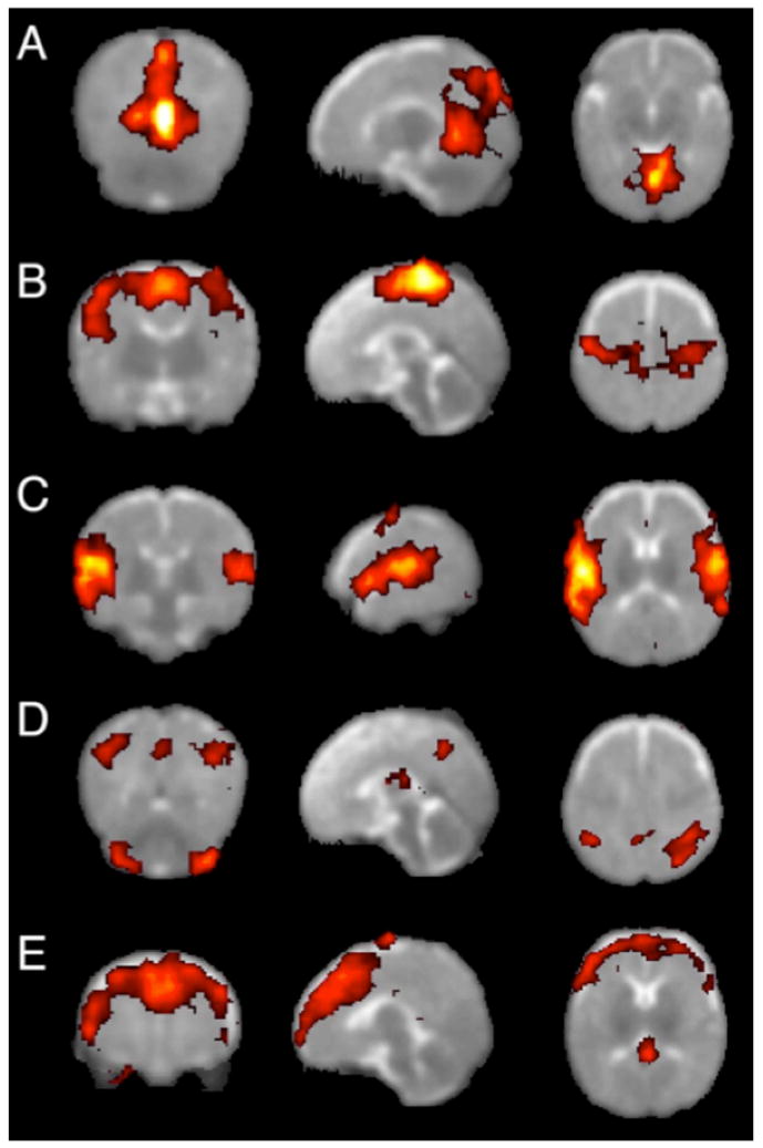
Group resting-state components in 12 sedated preterm infants. Each row shows coronal, sagittal, and axial view of components thresholded at P>0.5 (alternative-hypothesis threshold for activation vs null). (A) primary visual cortex,(B) bilateral somatosensory and motor cortex, (C) bilateral temporal/inferior parietal cortex encompassing primary auditory cortex, (D) posterior lateral and midline parts of parietal cortex and lateral cerebellum, (E) medial and lateral anterior prefrontal cortex. Figure modified from (Fransson et al., 2007).
These studies used both seed correlation maps and component maps to usefully demonstrate spatial features of correlated rs-fcMRI signal, but they also reveal limitations inherent to such approaches. For example, if one is interested in multiple regions highlighted in a seed correlation map, a new map needs to be generated for each additional region, and comparing more than a few maps at once quickly becomes overwhelming. Alternatively, if one is interested in interactions within or between components, one must adopt some other technique to examine those interactions, since component analyses only indicate that variance is shared to some extent by voxels within components. Such problems are amplified when multiple cohorts are examined (e.g. clinical or developmental cohorts), imposing substantial limits on the complexity and scope of brain relationships that can be grasped and communicated by researchers using these methods. Such limitations suggest the need for a more comprehensive framework for analyzing interactions between brain regions.
STUDIES OF RESTING STATE RELATIONSHIPS IN OLDER CHILDREN
Similar to the studies in younger children, several recent studies have examined rs-fcMRI correlation patterns in older children, and many of these studies have particularly or tangentially targeted the state of functional connectivity within the default mode network (DMN) over development, with both common and disparate results.
Fair et al. (Fair et al., 2008) examined functional connectivity between 13 published ROIs from the DMN over development in healthy subjects 7–30 years old. Here, ROIs were modeled as 10 mm diameter spheres, and functional connections were measured by Pearson correlations between ROI timecourses. A principal finding of this study is shown in Figure 2. At a chosen threshold (r > 0.15), networks in children ages 7–9 years existed in 5 unconnected pieces (Figure 2A), whereas in young adults 21–31 years old the networks formed an integrated DMN (Figure 2B). Nearly all developmental changes in correlation strengths among these ROIs were increases (see Figure 2C insets, far right), and increases largely occurred in an anterior-posterior orientation (Figure 2C). One interesting point to note is that the sole long-distance anterior-posterior correlations present in children linked medial prefrontal cortex (MPFC) and superior frontal nodes to lateral parietal and posterior cingulate (PCC) and retrosplenial nodes (Figure 2A). This result was mirrored in MPFC seed correlation maps that showed only sparse correlations to the PCC, superior frontal, lateral parietal, and lateral temporal cortex in children, but robust correlations in adults. The level of connectivity in anterior-posterior directions, and in particular the degree to which connectivity with the DMN is present and coherent in children, is a subject of debate and intense investigation (see below).
Figure 2.
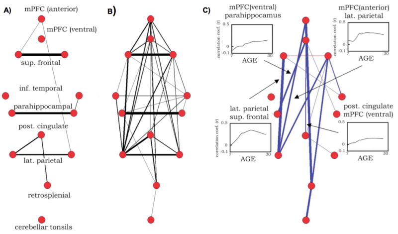
Pseudo-anatomical layouts of a network of 13 DMN ROIs in (A) children 7–9 years old and (B) adults 21–31 years old. Connection widths indicate the strength of correlation between ROI timecourses, and only correlations of r > 0.15 are shown. (C) The results of a two-tailed t-test of children and adult correlations corrected for multiple comparisons at P < 0.05. Correlations that increased with age are shown in blue, and those that decreased with age are shown in red. Insets show LOWESS curves of several individual connections over development. ROIs were defined from (Fox et al., 2005). Figure modified from (Fair et al., 2008).
Partially consistent findings were reported by Kelly et al., who studied correlation maps from 5 sequential seeds placed along the anterior cingulate (thought to participate in 5 different functional domains) in cohorts ages 9–13, 13–17, and 20–24 years (Kelly et al., 2009). Correlation maps in the youngest cohort displayed diffuse correlations near seed locations and few long-distance correlations. Over adolescence, however, correlations proximal to seeds tended to weaken, and correlations at long distances began to emerge, consistent with previous reports of functional connectivity development (Fair et al., 2007a). This pattern was most pronounced in ventral cingulate seeds (classically placed in the DMN), and least pronounced in dorsal seeds near the supplementary motor area (SMA). In particular, and in contrast to the findings of Fair et al. (Fair et al., 2008), Kelly et al. reported a complete absence of anterior-posterior midline correlations from ventral cingulate seeds in their youngest cohort, which increased over development to form full default-like correlation maps in adults.
Several ICA studies in older children have focused on the DMN. Thomason et al. used group ICA in 9–12 year olds to identify a default-like component that included PCC, MPFC, and bilateral lateral parietal regions, and produced a seed correlation map from PCC that mimicked the default-like component structure (Thomason et al., 2008). Supekar et al. also used ICA to identify a similar default-like component in cohorts of 7–8 and 19–22 year olds (Supekar et al., 2010). This study found significant and increasing partial correlations between PCC and MPFC over development, but minimal partial correlations between PCC and bilateral medial temporal lobe (MTL) in children, which became very weak partial correlations in adults. An additional study by Stevens et al. used ICA/PCA analyses to define 13 components in subjects ages 12–30 years, several of which resembled the default mode network, but since group ICA was performed on all subjects at once, it is unclear to what extent component structures reflect patterns found in children, adolescents, or adults (Stevens et al., 2009).
Overall, results pertinent to the DMN from several studies indicate that 1) in two studies, Fransson et al. (Fransson et al., 2009; Fransson et al., 2007) found no DMN-like component in infants, and no significant correlations between frontal and parietal components, though the parietal component contained midline and lateral parietal cortex, similar to the posterior portion of the DMN, 2) Smyser et al. (Smyser et al., 2010) found only insignificant MPFC-PCC correlations in their preterm infants, but significant MPFC-PCC correlations were found in some term infants, 3) Gao et al. (Gao et al., 2009) reported components in neonates that were distributed and which somewhat resembled portions of the DMN, 4) Kelly et al. (Kelly et al., 2009) found no anterior-posterior correlations from ventral ACC seeds in children 9–13, and noted substantial increases in long-distance correlations from these seeds throughout adolescence, 5) Fair et al. (Fair et al., 2008) detected sparse but significant correlations from an MPFC seed to PCC in 7–9 year olds, but most DMN ROIs in children lacked strong correlations with one another, and changes in correlation strengths within the DMN were almost all positive over adolescence, 6) Thomason et al. (Thomason et al., 2008) produced a default-like ICA component and seed correlation map from the PCC in children 9–12, and 7) Supekar et al. (Supekar et al., 2010) also produced a default-like ICA component in children 7–8 years old, and reported significant partial correlations between PCC and MPFC in their young cohort, which increased over development.
Though there appears to be a developmental trajectory towards increased functional connectivity within the DMN over development, the level of maturity within this system at any given age is unclear. One might conclude that coherence within the DMN is absent, weak, moderate, or strong in older children, depending upon the methodology used and the significance criteria employed. Differences in individual connections between DMN regions appear quite salient when the DMN is considered in isolation, but the functional network of the brain encompasses much more than just the regions of the DMN. If DMN regions in children are immature pieces of an adult network waiting to be wired together, then placing the DMN in a wider network context will reveal that DMN regions weakly interact with other brain regions in children but come to interact strongly with other DMN regions by adulthood, and we are right to attend closely to individual connections within the DMN over development. On the other hand, if a wider network context reveals that DMN regions actually interact with different sets of brain regions in infants and children than in adults, then targeted studies of DMN regions will miss these interactions by definition, and may miss the forest for the trees.
These considerations suggest the need for more comprehensive studies of functional networks over development, but as we described earlier, traditional seed-based and component-based analyses become inordinately complicated when many cohorts or components/ROIs are studied. This line of argument further suggests the need for a more powerful framework from which to study functional brain networks. Such a framework may be found in graph theory.
A RATIONALE FOR GRAPH THEORETIC APPROACHES TO MRI NETWORKS
The study of networks is an established and rapidly evolving multidisciplinary field, spearheaded by a branch of mathematics called graph theory (of note, networks are also called graphs). In graph theory terms, a network is a collection of items (called nodes or vertices) that possess pairwise relationships (called edges). Over the last 15 years, the increased availability of large, high-quality datasets has fundamentally changed how networks are understood and modeled. To name one example, in 1999 Barabasi and colleagues reported the presence of a surprisingly large number of highly connected nodes (called hubs) in the World Wide Web (Albert et al., 1999). This finding was at odds with classical models of network structure and growth, and spurred interest in “preferential attachment” models of network growth (Barabasi and Albert, 1999), in which nodes joining a network preferentially attach to well-connected nodes, rather than randomly connecting to the network. Preferential attachment makes intuitive sense in many situations (consider the first-publisher advantage in citation networks (de Solla Price, 1965; Newman, 2009)), and indeed variants of this model appears to generally capture the behavior of several real-world networks (Barabasi and Albert, 1999; Price, 1976). This line of research also led to the realization that the presence and frequency of hubs has strong implications for network integrity under attack (Albert et al., 2000), a finding with clear relevance to epidemiologists, the military, and neurologists.
An exciting pattern emerging from graph theoretic studies is that discoveries made in specific networks often generalize to other networks. For example, Watts and Strogatz first described the small-world architecture (discussed below) in the U.S. power grid, the C. elegans neural network, and a network of film actors (Watts and Strogatz), but this property has now been reported in hundreds, if not thousands, of other datasets. Such similarities suggest that complex networks may be governed by fundamental, knowable principles, and that discoveries made in one field may well apply to networks in other fields. This generalizability strongly suggests that neuroscientists studying the brain should be interested in the properties of other real-world and model networks. Accordingly, rs-fcMRI studies can leverage a substantial graph theoretic literature to explore the properties of functional brain networks, such as which nodes are critical for information flow or network integrity, which parts of functional networks are better structured for local versus global processes, and what types of processes could give rise to observed network structures. Recent graph theoretic studies have begun to explore such issues in adult brain networks (for review, see Bullmore & Sporns, 2009 (Bullmore and Sporns, 2009)), and here we focus on studies that examine functional networks in children (often in comparison with adults). This review will introduce several aspects of graph theory in the following section, but interested readers are referred to Newman, 2010 (Newman, 2010) for a fuller introduction to the field, and to Rubinov, 2009 (Rubinov and Sporns, 2009) for a discussion of graph theoretic measures in the context of MRI data.
GRAPH THEORY: A BRIEF PRIMER
A brief discussion of common practices and ground principles will aid the reader in digesting the data to come, and will illustrate the power of graph theoretic approaches to analyzing networks. This section will define graphs, and then introduce tools for visualizing graph structure, for probing the sub-structure of graphs, for describing large-scale attributes of graphs, and for finding and describing interesting nodes or collections of nodes within graphs. We ask for the reader’s patience in this somewhat abstract section. All concepts introduced will subsequently be applied to developmental data. It is our contention that these tools overcome many of the limitations of seed-based and component-based network analyses, and will enable us to reexamine some of the previously described developmental data in a clarifying light.
Graphs, nodes, edges, and the adjacency matrix
To reiterate, networks are collections of items that possess pairwise relationships. Graphs represent these items and relationships as nodes and edges. The structure of a graph is fully described as a list of nodes and the edges between nodes, and this structure can be conveniently organized as a matrix, called an adjacency matrix, in which each node has a column (and a row) of entries describing that node’s relationship to itself and to all other nodes (see Figure 3A). In fcMRI studies, nodes represent voxels or collections of voxels, and edges between nodes are typically similarity measures between node BOLD timecourses. Thus, a representative fcMRI graph might be a cross correlation matrix derived from the fcMRI timecourses of a collection of regions of interest (ROIs). Edges in such networks have values between −1 and 1, and the values of edges are called edge weights. Adjacency matrices fully describe the structure of a graph, and are the substrate for graph theoretic analyses, but it is difficult to comprehend the structure of a network by inspecting a matrix. We now describe a method of visualizing networks.
Figure 3.

(A) The adjacency matrix of a model 22-node graph. For any two nodes, the value of the edge between them (here a 1 or 0), is found at the intersection of the respective row and column (or vice versa) of each node. For example, matrix entry (2,3) shows a value of 1, which is the edge between node 2 and node 3. (B) A spring-embedded layout of the graph, where nodes are circles, and edges are lines between the nodes. (C) A list of several node properties. We illustrate several principles with this figure: the degree of node 20 is 3, because it has 3 edges (to nodes 5, 16, and 22). These nodes are the neighbors of node 20. The clustering coefficient of this node is 0/3, since the neighbors share no edges, out of 3 possible edges. In contrast, the clustering coefficient of node 5 is 1/3. The minimum path length is the number of edges that must be crossed to travel between two nodes. In the case of nodes 2 and 18 (red arrows), the minimum path length is 4 (2-3-6-22-18). The characteristic path length and average clustering coefficient are simply the average of all minimum path lengths and clustering coefficients across the network. The values of this network, in comparison to random and regular graphs, indicate a small-world structure. The betweenness centrality of a node is (proportional to) the fraction of all shortest paths in the network that run through the node. The value for node 1 is 0, whereas the values for nodes 6 and 22 are among the highest in the network, since paths from green to blue nodes almost always use these nodes. High degree and betweenness centrality values are often used to identify hubs, but these values do not necessarily correlate with each other, and must be used with caution, as illustrated by comparing the properties of node 2 with node 18 (values circled in red). Node 2 has a relatively high betweenness centrality, despite the fact that it is evidently not playing a “central” role in the network. This “discrepancy” is because all shortest paths to node 1 must traverse node 2, inflating its betweenness centrality. Contrast the network position of node 2 with that of node 18, which has a much higher degree but only slightly higher betweenness centrality, or node 9, which has high degree but quite low betweenness centrality. Community structure is visually evident in this layout, and modularity-optimizing algorithms obtain the partition indicated by node colorings, which yields a “modularity” of 0.54. Modularity values above 0.3 are typically thought to indicate strong community structure.
Visualizing a network: spring embedding layouts
Spring embedding techniques attempt to visualize a network in a “natural” state. Typically, nodes are randomly placed in space, and edges are placed between nodes. Edges are modeled as springs, with attractive forces proportional to edge weights. A global repulsive force is added to the system, and an energetic cost is calculated. Nodes iteratively reposition, and the system is allowed to cool to an energetic minimum. Though local minima and multiple layout solutions are possible, the resulting visualizations conveniently represent the network structure, such that connected nodes tend to lie close to one another and far from nodes to which they have no edge. Though the technique is qualitative, it is much more accessible than examining adjacency matrices, and the complicated structures of networks with dozens to hundreds of nodes can be easily and quickly apprehended (Figure 3B). Additionally, though it is not actually necessary to visualize a network in order to understand it, visual inspection can facilitate an intuitive understanding of properties that may be quantified by other means. For example, Figure 3 shows the adjacency matrix and a spring-embedded layout of a graph containing several dozen nodes. It is visually evident that the network is clumped in certain areas where nodes are richly connected, a property that can be quantified using measures of community structure.
Global network properties: community structure and the small-world structure
Communities (also called modules) within networks are groups of nodes that are richly connected to one another within the larger framework of the entire network. Communities have been detected in many complex networks, and tend to group nodes with similar features or functions, simplifying and illuminating the structure of the network (for review, see Fortunato, 2010 (Fortunato, 2010)). Community detection has been the subject of intense interest since 2004, when Newman & Girvan proposed the “modularity” measure, which quantifies the “quality” or amount of community structure found in a network (Newman and Girvan, 2004). For a given partition of a graph into modules, the modularity of the graph is the difference between the number of edges found within modules and the number of edges predicted to lie within modules if all edges in the network were distributed randomly (Newman and Girvan, 2004). Algorithms that optimize this measure have been widely used to detect communities in networks, though several alternatives exist (see Fortunato, 2010).
Graphs are, in a reductive sense, nothing more than a collection of nodes and edges. This is, however, like saying that a symphony is just a collection of notes. Networks formed from identical numbers of edges and nodes can have starkly differing properties depending upon the patterning of edges in the network (as we will see shortly), and a cardinal virtue of graph theoretic approaches to networks is that they can not only describe network structures, but they can also interpret these structures to reveal properties of networks and their nodes. We have already encountered one such measure, the “modularity” of a graph, which indicated the extent of community structure in a network. We now consider another fundamental property of graphs, which is how efficiently their structures facilitate local and global communication (by communication, we simply mean the passing of something, like a packet of information, from node to node over the network). Numerous methods have been proposed to capture this property in graphs (e.g. the “efficiency” and “cost-efficiency” measures (Achard et al., 2006; Latora and Marchiori, 2001)), and we focus on some of the most well-known, the “small-world” measures (Watts and Strogatz, 1998).
Given some number of nodes and edges, classic network models could create networks of two extremes: a regular graph in which all nodes had similar numbers of edges and connected with their nearest neighbors in a lattice-like structure, and a random graph, in which nodes had similar numbers of edges, but edges were distributed randomly throughout the graph. In a lattice, few edges were needed to communicate between nearby nodes, but many edges would be crossed to communicate with distant portions of the network. In a random graph, information could reach distant nodes using a small number of edges, but reaching nearby nodes required many more edges than on a regular lattice. Thus, regular graphs were locally efficient but globally inefficient, and random graphs were efficient for global but not local interactions.
These properties are captured in the characteristic path length and average clustering coefficient of networks (Figure 3C). Given a network in which all nodes can reach one another, at least one shortest path exists between all nodes, and one can calculate the characteristic path length as the average shortest path on the network, measuring how easily information can travel between distant nodes. The (local) clustering coefficient of a node is the ratio of edges present between the neighbors of a node (a node with 3 edges has 3 neighbors, see Figure 3) to the number of edges possible between neighbors of a node. This coefficient takes values between 0 and 1, where low coefficients indicate that few neighbors of a node are themselves neighbors, and high coefficients indicate that a node is embedded in a richly connected local environment. Thus, random graphs are characterized by low path lengths and low clustering coefficients, whereas lattices have high path lengths and high clustering coefficients.
The fundamental insight of the small-world structure, proposed by Watts and Strogatz, is that networks can possess both high clustering coefficients and low path lengths, making them simultaneously efficient on both local and global scales (Watts and Strogatz, 1998). Watts and Strogatz discovered that a regular lattice retained high clustering coefficients but drastically reduced average path lengths if a few edges of the lattice were randomly “re-wired”, creating short-cuts to distant portions of the network. This structure has been found in numerous real-world networks (including neural and MRI networks (Eguiluz et al., 2005; Humphries et al., 2006; Watts and Strogatz, 1998)), and comparisons between the “small-worldness” of networks can be made by normalizing observed small-world measures to those found in regular and random graphs with similar numbers of nodes and edges.
Local network properties: node degree, hubs and node betweenness centrality
The structure of a network confers properties not only on the network as a whole, but also upon individual nodes. The clustering coefficients just discussed are one such property, which measure how richly integrated the local environment around a node is (Figure 3C). Another set of measures of much practical use are measures of node centrality, which indicate to what extent a node plays a “central” or important role within a network. As with the measures for network efficiency, there are multiple methods to assay node centrality, and we highlight two of the simplest here.
One method to measure node centrality is simply to sum all edges connected to a node. This is known as the “degree centrality”, or simply the degree, of a node (Figure 3). High-degree nodes are called hubs, and can play important roles in network structure and dynamics. The second method is to calculate the fraction of all shortest paths in a network that cross over a given node (or edge). This proportion is the “betweenness centrality” of a node (or edge), which is a useful measure of how much information might traverse certain parts of a network, presuming that optimal paths are used. High values can identify nodes that are crucial bridges between communities and/or possible bottlenecks in network traffic, and may also identify hubs. The measure must be used with caution, however, since it may also yield high values at the periphery of networks if peripheral nodes have few possible paths into the main body of the graph (see Figure 3, node 2). These measures of centrality have been used for many purposes, one of which has been to identify hubs within MRI networks (Buckner et al., 2009; Hagmann et al., 2008).
The importance of thresholding and edge density
We make a final technical point before turning to data. In rs-fcMRI networks, the similarity measures used to define edges (often Pearson or partial correlations) yield weights on the edges. For example, in networks formed from correlation matrices, all nodes relate to all other nodes with edges weighted −1 to 1. Negative edges are mathematically troublesome in many graph analyses, and edges with weights near zero are likely to be uninformative, and so a threshold is often applied to networks, eliminating edges with weights below the threshold. As thresholds rise, the density of edges in the network decreases, and at some point the network will begin to fragment into disconnected components. The actual structure of the network changes as edges are removed, and thus many network properties are functions of edge density. Additionally, there is no “correct” edge density or threshold at which to examine a network. For this reason, when investigating some property of interest, network studies should report results over a range of thresholds or edge densities to demonstrate this relationship, as well as the reliability of the findings. Typical threshold ranges begin at or above zero, to avoid negative and/or weak edges, and stop once the graph begins to fragment into components. When comparing the properties of two or more networks (e.g. networks from multiple developmental cohorts), it is useful to control for edge density, so that differences in network properties do not arise from differences in graph density. There is no agreed-upon method for comparing network properties, but common methods include simple non-statistical comparisons, t-tests of values at particular edge densities between cohorts, and comparison of parameters derived from growth curve fits of properties vs. threshold (Supekar et al., 2009).
These measures are a small sampling of the tools available in graph theoretic analyses, but serve to illustrate the versatility and comprehensiveness of a graph theoretic approach to networks. We will encounter each of these tools in the coming studies, and we now turn to applications of these techniques to rs-fcMRI data.
INITIAL GRAPH THEORETIC STUDIES OF DEVELOPMENT
Graph theory was introduced to developmental studies of functional networks in a series of reports by Fair et al., beginning in 2007 (Fair et al., 2007a). Here, 39 published task control ROIs (Dosenbach et al., 2006) that were defined in young adults were examined in a developmental cohort. A previous study had examined these ROIs as a graph in adults and reported that, at many thresholds, the graph existed as two disconnected components (Dosenbach et al., 2007) (components in graph theory are disconnected pieces of the graph, not ICA or PCA components), meaning that nodes within one component had no correlations over a particular threshold to nodes in the other component. These components were termed the cingulo-opercular (CO) and fronto-parietal (FP) task control networks, based on the locations of their constituent ROIs. Each component tended to have different functional properties in fMRI studies, such that ROIs in the CO network tended to display sustained activity during tasks, while ROIs in the FP network tended to activate more transiently, linking the functional properties of ROIs to their properties as nodes within rs-fcMRI networks. Children and adults differ behaviorally in task performance (Brown et al., 2005; Church et al., 2010; Schlaggar et al., 2002), and fMRI studies have documented developmental differences in activity in task control regions during task performance (Velanova et al., 2009), leading Fair et al. to examine task control regions for developmental changes in functional network structure. To accomplish this, 39 task control regions were examined as graphs in rs-fcMRI data from 210 subjects ages 7–35 years. Nodes were formed by modeling ROIs as 10 mm diameter spheres, and edges were defined as the Pearson correlations between node rs-fcMRI timecourses.
The graph theoretic analysis of these networks was straightforward, and simply involved visualizing the graphs in a pseudo-anatomic layout and examining their structure, shown in Figure 4. In children ages 7–9 years, the graph was a single component, the dorsal anterior cingulate/medial superior frontal cortex (dACC/msFC) node was embedded within the FP nodes, and the bilateral anterior prefrontal cortex (aPFC) nodes bridged between FP and CO groupings (Figure 4A). In adolescents ages 10–15 years, the graph broke into two components, but the dACC/msFC node remained in the FP component (Figure 4B). In adults ages 21–31 years, the graph existed as 2 components corresponding to the FP and CO task control networks, as expected (Figure 4C). Thus, the network reorganized over development, such that anterior cingulate and aPFC nodes dissociated from other frontal nodes to more strongly associate with insular and thalamic nodes. The authors also measured the Euclidean distance between all pairs of ROIs, and noted that short-distance edges tended to be strong in children and weaken over development, whereas long-distance edges tended to be weak in children and strengthen over development, a trend that has been replicated in several studies, using both Euclidean and DTI-based distances (Fair et al., 2009; Kelly et al., 2009; Supekar et al., 2009).
Figure 4.
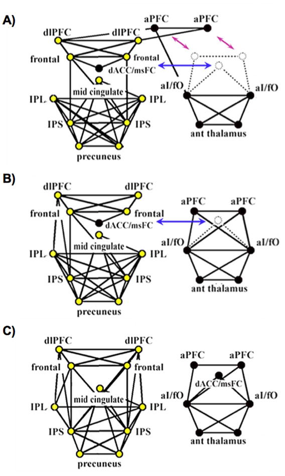
The 39-node task control graphs of Fair et al, 2007. Fronto-parietal nodes are colored in yellow, and cingulo-opercular nodes are colored in black. Graphs are portrayed in a pseudo-anatomical layout at 10% edge density. (A-C) show graph structures in children ages 7–9 years, adolescents ages 10–15 years, and adults ages 19–31 years, respectively. Note the shifting associations of aPFC and dACC/msFC nodes, and the emergence of greater frontal-parietal functional connectivity over development. ROIs and node memberships were defined in (Dosenbach et al., 2006) and (Dosenbach et al., 2007). Figure modified from (Fair et al., 2007a).
A subsequent study by Fair et al. (Fair et al., 2009) used spring embedding layouts to examine the development of a network composed of 34 published default, task control, and error-responsive ROIs (Dosenbach et al., 2007; Dosenbach et al., 2006; Fair et al., 2007a; Fox et al., 2005). Nodes, edges, and subjects were defined as before. Figure 5 shows layouts of the graphs at several ages. Two striking patterns are noted. First, nodes that are anatomically proximal tend to have strong correlations in children, which weaken over development (the light-blue-rimmed frontal lobe nodes of Figure 5A). Second, nodes that are functionally related in adults are not strongly associated in children, but come to associate strongly over development (e.g. the red-filled DMN nodes of Figure 5B). The patterns of edges clearly change across ages, and it is evident that the network is clumped in certain areas where nodes are densely connected, indicating that the network possesses community structure.
Figure 5.

The 34-node graphs of task-control, default, and error-related (cerebellar) ROIs of Fair et al, 2009. Graphs are presented in spring embedded layouts at average ages 9, 13, and 25 years moving from left to right. Node centers are colored by pre-defined functional system membership (i.e. all red nodes represent published DMN coordinates), and node rims are colored by anatomical location within the brain (e.g. all blue rims indicate nodes in frontal cortex). The blue clouds (A) highlight the location of frontal nodes across development, and the red clouds (B) highlight the location of pre-defined default mode regions over development. ROIs and node memberships were defined in (Dosenbach et al., 2007; Dosenbach et al., 2006; Fair et al., 2007a; Fox et al., 2005). Figure modified from (Fair et al., 2009).
A modularity-optimizing community detection algorithm was applied to this network, and strong community structure was detected at all ages examined, consistent with the spring embedded layouts. Interestingly, the modularity value attained by the algorithm did not change (qualitatively) over age, indicating that the “quality” of community structure was similar (and high) in children, adolescents, and adults. Importantly, however, the composition of modules did change over development. In children, modules grouped nodes largely by anatomical location, whereas modules in adults grouped nodes almost perfectly by their functional role (default, fronto-parietal, cingulo-opercular, and cerebellar error categories).
This study also calculated the small-world properties of these graphs, and found that throughout development from childhood to young adulthood, network clustering coefficient values were near those of lattices, and network path length values were near those of random graphs, indicating that the graphs were small-world networks at all ages examined. This suggested that despite the large differences in community structure across development, that child, adolescent, and adult networks were all organized in a manner that facilitated simultaneous efficiency on local and global scales. Edge density was not held constant in this analysis for small-world comparisons, but subsequent studies have replicated this finding while controlling for edge density. Supekar et al. reported small-world structure in both child and adult whole-brain graphs, but found no significant differences between them (Supekar et al., 2009). Similarly, Fransson et al. reported small-world architectures in both infant and adult voxelwise graphs, though direct comparisons between graphs were not possible (Fransson et al., 2010).
LESSONS FROM GRAPH THEORETIC INVESTIGATIONS OF NETWORK STRUCTURE AND PROPERTIES
These studies suggest several tentative conclusions. First, selected short-distance edges tend to be strong in children and to weaken over development, in contrast to a subset of long-distance edges, which are typically weak in children, and which increase in strength over development. Second, these developmental increases in edge strengths tend to occur between nodes that are functionally related in young adults, such as edges between nodes within the default mode network, or edges between nodes of the fronto-parietal task control network. Third, community structure is present and strong in graphs at all stages of development. Fourth, as a result of local decreases and long-distance increases in edge strengths over development, communities in children group nodes largely by anatomical proximity, whereas communities in adults group nodes by functional roles. Finally, despite the reorganization of communities over development, graphs are consistently structured in manners that facilitate efficiency at both local and global network scales.
These conclusions must be tempered by several caveats. First, for the most part, the graph structures of functional networks in any one study have only been described at limited ages, and only within limited subsets of brain regions. Future networks should extend networks to include other brain regions to examine developmental trends more comprehensively. Second, only limited comparisons of network properties have been made thus far. Statistical comparisons were not made in small-world properties by either Fair et al. (Fair et al., 2009) or Fransson et al. (Fransson et al., 2010), and Supekar et al. (Supekar et al., 2009) made comparisons at only a single edge density. Thus, rigorous examinations of differences in network properties such as the small-world measures have not yet been performed. Confirmation and extension of these results awaits studies that examine influences of both threshold and edge density while examining larger, brain-wide functional networks over development from infancy through adulthood.
However, an important lesson already apparent from these studies is that functional networks examined in isolation may appear quite different when examined within wider network contexts. We noted differential reports of functional connectivity within the DMN earlier in this review. Some studies, such as those of Fair et al. (Fair et al., 2008) or Kelly et al. (Kelly et al., 2009), suggested absent to minimal connectivity within the DMN in older children, whereas studies by Supekar et al. (Supekar et al., 2010) and Thomason et al. (Thomason et al., 2008) suggested substantial DMN connectivity at similar ages. In isolation, these differences appear quite striking. However, once the DMN is placed in a larger network with other cortical regions, it becomes clear that DMN regions are not isolated fragments of an immature adult functional system, nor are they unified in a cohesive DMN, but rather that DMN regions are actually integrated into a different network structure in children than adults (Fair et al., 2009). Communities in children are organized by anatomical proximity, suggesting that the various parts of the DMN should be considered as participants in relatively separate functional modules, not as fragmented elements of an adult functional system. Naturally, a transition to adult-like structures must occur over development, as long-distance connections between PCC, MPFC, and other regions of the DMN strengthen, and short-distance relationships weaken. Yet to focus upon these internal changes without considering external relationships risks fundamentally misapprehending the developmental trajectory of the adult DMN regions.
GRAPH THEORETIC INVESTIGATIONS OF NODE PROPERTIES
In the previous section, graph theoretic approaches were used to describe the structure and properties of entire networks. We now examine two studies that used graph theoretic approaches to identify individual nodes that might play important roles in functional brain networks. The results of these studies highlight, among other things, the complexity of interpreting network studies, and the need for comprehensive presentation of data.
Fransson et al. (Fransson et al., 2010) used measures of degree and betweenness centrality to identify the location of network hubs in voxelwise networks in infants and adults, in a manner similar to recent studies in adults (Buckner et al., 2009; Sepulcre et al., 2010). As shown in Figure 6, the locations of hubs identified using either degree or betweenness centrality were quite similar within cohorts, but differed substantially between cohorts. In adults (Figure 6C,D), many hubs appear to lie in the DMN, whereas in children (Figure 6A,B), many hubs appear to lie in or near primary sensorimotor cortex. It is not immediately obvious why such close correspondence should exist between measures of degree and betweenness centrality, though similar findings have been previously reported (Buckner et al., 2009). Degree is a property of a single node regardless of its position in a network, whereas node betweenness centrality is highly dependent upon a node’s location within the network structure (e.g., two nodes of identical degree can have very different betweenness centralities if one is locally embedded within a module and the other bridges between modules, see Figure 3), and thus it is somewhat surprising that these measures should correspond so closely in these voxelwise networks.
Figure 6.
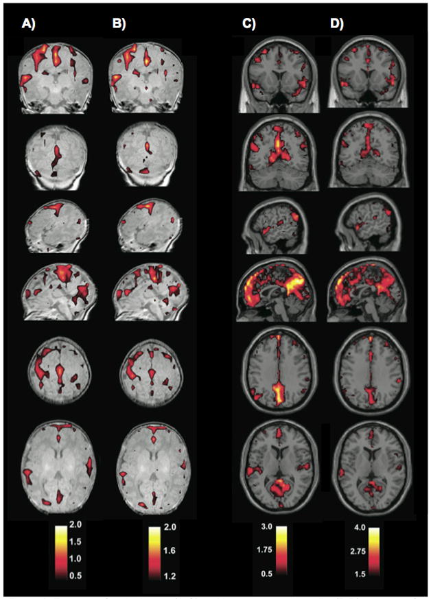
Node degree (A,C) and betweenness centrality (B,D) z-scores of voxels in voxelwise graphs in infants (A,B) and adults (C,D). Calculations were performed on adjacency matrices that were thresholded at 0.3, and then binarized. Note the congruence between the two measures within children or adults, but the evident differences between children and adult patterns. Figure adapted from (Fransson et al., 2010).
One possible explanation for the similarity between degree and betweenness centrality runs as follows. Studies in adults have demonstrated that voxels within putative functional areas possess similar rs-fcMRI timecourses (Cohen et al., 2008). Functional areas within functional systems (e.g. the various portions of the DMN) tend to have correlated rs-fcMRI activity, and thus voxels should generally possess a) strong correlations within their functional area, and b) moderate correlations to functionally-related functional areas. In voxelwise graphs, this scenario could give rise to a hierarchical modular structure of functional areas and functional systems, and a voxel’s degree would generally scale 1) with the size of its functional area, and 2) with the number (and sizes) of functional areas comprising its functional system. Stated differently, a voxel’s degree should scale with the size of its module. If the default module spanned the greatest number of voxels in adults, it would be unsurprising that the highest-degree voxels in adults would be identified within default-like regions. “Hubs” in this scenario are simply members of the largest (whether measured by nodes, voxels, or volume) graph module. Similarly, if this module occupied either a very central or very peripheral role in the overall graph, voxels within the module would tend to have high betweenness centralities (Figure 3). Similar arguments apply to the sensorimotor hubs of infants. Placement of hubs into a graph layout could reveal the reason for the congruence between degree and betweenness centrality, but without such information, it is difficult to evaluate the meaning of these findings, though they clearly indicate differences in the functional network structures of infants and adults.
In a different study, Gao et al. (Gao et al., 2009) used a similar strategy to identify hubs in default-like components in young children, and calculated betweenness centrality on networks of 6, 13, 19, and 7 nodes in cohorts of neonates, 1 year olds, 2 year olds, and adults, respectively. Each cohort returned the highest betweenness centrality in the PCC, but it is questionable whether such techniques are truly meaningful in networks of only 6 or 7 nodes, since the addition or deletion of a single edge could substantially alter many shortest path lengths.
These studies highlight a fundamental issue in MRI graph theoretic studies, which is the extent to which an abstract network is constructed to reflect the functional network structure of the human brain. In many systems, nodes are obvious, such as stations along subway lines, or people who have coauthored papers. Nodes are, however, not obvious in the functional network of the brain. Presumably, when studying the functional network architecture of the brain, nodes should correspond to some unit of functional organization, such as neurons, columns, or functional areas. Unfortunately, the number, locations and extents of such functional units in the human brain are poorly defined at this point, and researchers therefore typically form nodes from voxels (Buckner et al., 2009; Eguiluz et al., 2005; van den Heuvel et al., 2008), pre-defined anatomical brain parcellation schemes (Achard et al., 2006; He et al., 2009; Meunier et al., 2009; Salvador et al., 2005), or pre-defined ROIs, often obtained from fMRI or fcMRI studies (Church et al., 2009; Dosenbach et al., 2007; Nelson et al., 2010). If the brain is a collection of functional units such as columns or functional areas, then nodes defined by undersampling, oversampling, or merging such units will necessarily result in a network that distorts, to some extent, the true composition of the brain’s network, and networks must be examined and interpreted accordingly.
CONCLUDING REMARKS
A broad theme that emerges from these studies of functional networks is that at young ages, ROIs tend to have strong rs-fcMRI signal correlations with nearby ROIs, and that over childhood and adolescence, selected local correlations tend to weaken, while correlations with more distant ROIs tend to increase. This trend is evident in the increased seed map bilaterality with gestational age seen in the infants of Smyser et al. (Smyser et al., 2010), in the increased extents of sensorimotor correlation maps of Lin et al. in young children (Lin et al., 2008), and in the increases of edge strengths within the graphs of Supekar et al. (Supekar et al., 2009) and Fair et al. (Fair et al., 2009) over late childhood and adolescence. In the anterior cingulate, Kelly et al. (Kelly et al., 2009) specifically note that this trend is least pronounced in seeds near SMA, and occurs latest and most markedly in ventral seeds typically associated with the DMN. This trend likely stems from several sources. Synaptic pruning takes place throughout the first twenty years of life (Huttenlocher, 1979), and could contribute to reduced local rs-fcMRI correlation. Conversely, myelination throughout childhood and adolescence could facilitate increased long-range rs-fcMRI correlations (Brody et al., 1987; Paus et al., 2001). Computational and empirical studies have demonstrated significant correlations between structural and functional connectivity (Hagmann et al.; Honey et al., 2007), giving support to such ideas, though they have also demonstrated that present estimates of structural connectivity leave much of the variance in rs-fcMRI signal unaccounted for (Honey et al., 2009).
An additional theme is that developmental increases in functional connectivity tend to take place between portions of the brain that are functionally related in adults. This trend is most apparent in the network structures of task control and default networks in multiple studies by Fair et al. (Fair et al., 2008; Fair et al., 2009; Fair et al., 2007a), the seed maps of Kelly et al. (Kelly et al., 2009), and in the increasing partial correlations within the DMN noted by Supekar et al. (Supekar et al., 2010). Neuronal firing patterns are known to modify synaptic weighting (Miltner et al., 1999), and one possible explanation for the increases in coherent rs-fcMRI signal between functionally related brain regions is that the signal arises from shared histories of spontaneous or evoked activity. Recent studies have demonstrated that visual perceptual learning can influence rs-fcMRI signal in adults, lending credence to this hypothesis (Lewis et al., 2009). On the other hand, rs-fcMRI signal correlations may facilitate shared processing between brain regions, and may actually participate in the development of the functional capabilities of brain circuitry (Bi and Poo, 1999; Fiser et al., 2004; Varela et al., 2001).
What is the benefit of increased long-range and/or decreased short-range rs-fcMRI correlations? At present, we can only speculate. It is plausible, and even probable, that increases in coherent activity within functional systems might facilitate particular cognitive abilities. In adults, rs-fcMRI correlations and network properties have been linked to measures such as IQ or task performance (Seeley et al., 2007; van den Heuvel et al., 2009). We are unaware of any developmental studies examining such relationships. Unfortunately, over childhood and adolescence, changes in functional connectivity will likely correlate with many behavioral or physiologic measures, such as height or hormonal levels, as well as various cognitive measures. Developmental studies of correlates between rs-fcMRI measures and cognitive or behavioral measures will therefore need tightly constrained hypotheses, or large datasets that can achieve the power needed to tease apart such covariance.
A significant finding that emerged from recent graph theoretic studies in children is that developing functional networks are in some respects quite similar to adult networks. Graph theoretic measures indicate that brain networks throughout development possess community structure (Fair et al., 2009), and are organized in manners that facilitate efficiency on local and global network scales (Fair et al., 2009; Fransson et al., 2010; Supekar et al., 2009). The limited comparisons made of such network properties have reported no differences between children and adults. This set of observations suggests that network structures in children ought not to be viewed as simple precursors to adult-like configurations, but should be given serious attention as intact, operational functional networks with some similar properties but a fundamentally different structure than adult networks. The field awaits confirmation and extension of these findings with rigorous, comprehensive studies of brain functional networks across development.
Finally, we wish to underscore the utility of graph theoretic approaches to describing brain networks. Graph theory is a rigorous, established, and appropriate framework within which to examine MRI networks. The tools it offers are powerful and flexible, and neuroscientists have only begun to tap the substantial resources available for studying brain networks (http://sites.google.com/a/brain-connectivity-toolbox.net/bct/Home). Graph theoretic approaches sidestep many limitations of more traditional analysis techniques, and enable more complete studies of brain networks than have been previously feasible. The utility of examining more comprehensive brain networks is hopefully evident from the work we have reviewed. Though much progress has been made in recent years, it is clear that the task of understanding the development of the structure and properties of functional brain networks is only beginning.
Footnotes
Publisher's Disclaimer: This is a PDF file of an unedited manuscript that has been accepted for publication. As a service to our customers we are providing this early version of the manuscript. The manuscript will undergo copyediting, typesetting, and review of the resulting proof before it is published in its final citable form. Please note that during the production process errors may be discovered which could affect the content, and all legal disclaimers that apply to the journal pertain.
Literature Cited
- Achard S, Salvador R, Whitcher B, Suckling J, Bullmore E. A resilient, low-frequency, small-world human brain functional network with highly connected association cortical hubs. J Neurosci. 2006;26:63–72. doi: 10.1523/JNEUROSCI.3874-05.2006. [DOI] [PMC free article] [PubMed] [Google Scholar]
- Albert Jeong, Barabasi Error and attack tolerance of complex networks. Nature. 2000;406:378–382. doi: 10.1038/35019019. [DOI] [PubMed] [Google Scholar]
- Albert R, Jeong H, Barabasi AL. Internet: Diameter of the World-Wide Web. Nature. 1999;401:130–131. [Google Scholar]
- Barabasi AL, Albert R. Emergence of scaling in random networks. Science. 1999;286:509–512. doi: 10.1126/science.286.5439.509. [DOI] [PubMed] [Google Scholar]
- Bi G, Poo M. Distributed synaptic modification in neural networks induced by patterned stimulation. Nature. 1999;401:792–796. doi: 10.1038/44573. [DOI] [PubMed] [Google Scholar]
- Biswal B, Yetkin FZ, Haughton VM, Hyde JS. Functional connectivity in the motor cortex of resting human brain using echo-planar MRI. Magn Reson Med. 1995;34:537–541. doi: 10.1002/mrm.1910340409. [DOI] [PubMed] [Google Scholar]
- Biswal BB, Mennes M, Zuo XN, Gohel S, Kelly C, Smith SM, Beckmann CF, Adelstein JS, Buckner RL, Colcombe S, et al. Toward discovery science of human brain function. Proc Nat Acad Sci USA. 2010;107:4734–4739. doi: 10.1073/pnas.0911855107. [DOI] [PMC free article] [PubMed] [Google Scholar]
- Brody BA, Kinney HC, Kloman AS, Gilles FH. Sequence of central nervous system myelination in human infancy. I. An autopsy study of myelination. J Neuropathol Exp Neurol. 1987;46:283–301. doi: 10.1097/00005072-198705000-00005. [DOI] [PubMed] [Google Scholar]
- Buckner R, Sepulcre J, Talukdar T, Krienen F. Cortical Hubs Revealed by Intrinsic Functional Connectivity: Mapping, Assessment of Stability, and…. Journal of Neuroscience. 2009 doi: 10.1523/JNEUROSCI.5062-08.2009. [DOI] [PMC free article] [PubMed] [Google Scholar]
- Bullmore E, Sporns O. Complex brain networks: graph theoretical analysis of structural and functional systems. Nat Rev Neurosci. 2009;10:186–198. doi: 10.1038/nrn2575. [DOI] [PubMed] [Google Scholar]
- Carmichael ST, Price JL. Connectional networks within the orbital and medial prefrontal cortex of macaque monkeys. J Comp Neurol. 1996;371:179–207. doi: 10.1002/(SICI)1096-9861(19960722)371:2<179::AID-CNE1>3.0.CO;2-#. [DOI] [PubMed] [Google Scholar]
- Church JA, Fair DA, Dosenbach NU, Cohen AL, Miezin FM, Petersen SE, Schlaggar BL. Control networks in paediatric Tourette syndrome show immature and anomalous patterns of functional connectivity. Brain: A Journal of Neurology. 2009;132:225–238. doi: 10.1093/brain/awn223. [DOI] [PMC free article] [PubMed] [Google Scholar]
- Cohen AL, Fair DA, Dosenbach NU, Miezin FM, Dierker D, Van Essen DC, Schlaggar BL, Petersen SE. Defining functional areas in individual human brains using resting functional connectivity MRI. Neuroimage. 2008;41:45–57. doi: 10.1016/j.neuroimage.2008.01.066. [DOI] [PMC free article] [PubMed] [Google Scholar]
- Corbetta M, Shulman G. Control of goal-directed and stimulus-driven attention in the brain. Nature Reviews Neuroscience. 2002;3:201–215. doi: 10.1038/nrn755. [DOI] [PubMed] [Google Scholar]
- Corbetta M, Shulman GL, Miezin FM, Petersen SE. Superior parietal cortex activation during spatial attention shifts and visual feature conjunction. Science. 1995;270:802–805. doi: 10.1126/science.270.5237.802. [DOI] [PubMed] [Google Scholar]
- Cordes D, Haughton VM, Arfanakis K, Carew JD, Turski PA, Moritz CH, Quigley MA, Meyerand ME. Frequencies contributing to functional connectivity in the cerebral cortex in “resting-state” data. AJNR Am J Neuroradiol. 2001;22:1326–1333. [PMC free article] [PubMed] [Google Scholar]
- Cowan WM, Fawcett J, O’Leary DDM, Stanfield BB. Regressive events in neurogenesis. Science. 1984;225:1258–1265. doi: 10.1126/science.6474175. [DOI] [PubMed] [Google Scholar]
- Damoiseaux JS, Rombouts SA, Barkhof F, Scheltens P, Stam CJ, Smith SM, Beckmann CF. Consistent resting-state networks across healthy subjects. Proc Natl Acad Sci U S A. 2006;103:13848–13853. doi: 10.1073/pnas.0601417103. [DOI] [PMC free article] [PubMed] [Google Scholar]
- de Solla Price DJ. Networks of Scientific Papers. Science. 1965;149:510–515. doi: 10.1126/science.149.3683.510. [DOI] [PubMed] [Google Scholar]
- Dosenbach NUF, Fair DA, Miezin FM, Cohen AL, Wenger KK, Dosenbach RAT, Fox MD, Snyder AZ, Vincent JL, Raichle ME, et al. Distinct brain networks for adaptive and stable task control in humans. Proc Natl Acad Sci U S A. 2007;104:11073–11078. doi: 10.1073/pnas.0704320104. [DOI] [PMC free article] [PubMed] [Google Scholar]
- Dosenbach NUF, Visscher KM, Palmer ED, Miezin FM, Wenger KK, Kang HC, Burgund ED, Grimes AL, Schlaggar BL, Petersen SE. A core system for the implementation of task sets. Neuron. 2006;50:799–812. doi: 10.1016/j.neuron.2006.04.031. [DOI] [PMC free article] [PubMed] [Google Scholar]
- Eguiluz VM, Chialvo DR, Cecchi GA, Baliki M, Apkarian AV. Scale-free brain functional networks. Phys Rev Lett. 2005;94:018102. doi: 10.1103/PhysRevLett.94.018102. [DOI] [PubMed] [Google Scholar]
- Fair DA, Cohen AL, Dosenbach NU, Church JA, Miezin FM, Barch DM, Raichle ME, Petersen SE, Schlaggar BL. The maturing architecture of the brain’s default network. Proc Natl Acad Sci USA. 2008;105:4028–4032. doi: 10.1073/pnas.0800376105. [DOI] [PMC free article] [PubMed] [Google Scholar]
- Fair DA, Cohen AL, Power JD, Dosenbach NU, Church JA, Miezin FM, Schlaggar BL, Petersen SE. Functional brain networks develop from a “local to distributed” organization. PLoS Comput Biol. 2009;5:e1000381. doi: 10.1371/journal.pcbi.1000381. [DOI] [PMC free article] [PubMed] [Google Scholar]
- Fair DA, Dosenbach NUF, Church JA, Cohen AL, Brahmbhatt S, Miezin FM, Barch DM, Raichle ME, Petersen SE, Schlaggar BL. Development of distinct control networks through segregation and integration. Proc Natl Acad Sci U S A. 2007a;104:13507–13512. doi: 10.1073/pnas.0705843104. [DOI] [PMC free article] [PubMed] [Google Scholar]
- Fair DA, Schlaggar BL, Cohen AL, Miezin FM, Dosenbach NU, Wenger KK, Fox MD, Snyder AZ, Raichle ME, Petersen SE. A method for using blocked and event-related fMRI data to study “resting state” functional connectivity. Neuroimage. 2007b;35:396–405. doi: 10.1016/j.neuroimage.2006.11.051. [DOI] [PMC free article] [PubMed] [Google Scholar]
- Felleman DJ, Van Essen DC. Distributed hierarchical processing in the primate cerebral cortex. Cerebral Cortex. 1991;1:1–47. doi: 10.1093/cercor/1.1.1-a. [DOI] [PubMed] [Google Scholar]
- Fiser J, Chiu C, Weliky M. Small modulation of ongoing cortical dynamics by sensory input during natural vision. Nature. 2004;431:573–578. doi: 10.1038/nature02907. [DOI] [PubMed] [Google Scholar]
- Fortunato S. Community detection in graphs. Physics Reports. 2010;486:75–174. [Google Scholar]
- Fox MD, Snyder AZ, Vincent JL, Corbetta M, Van Essen DC, Raichle ME. The human brain is intrinsically organized into dynamic, anticorrelated functional networks. Proc Natl Acad Sci U S A. 2005;102:9673–9678. doi: 10.1073/pnas.0504136102. [DOI] [PMC free article] [PubMed] [Google Scholar]
- Fransson P, Aden U, Blennow M, Lagercrantz H. The functional architecture of the infant brain as revealed by resting-state fMRI. Cereb Cortex. 2010 doi: 10.1093/cercor/bhq071. [DOI] [PubMed] [Google Scholar]
- Fransson P, Skiöld B, Engström M, Hallberg B, Mosskin M, Aden U, Lagercrantz H, Blennow M. Spontaneous brain activity in the newborn brain during natural sleep--an fMRI study in infants born at full term. Pediatric Research. 2009;66:301–305. doi: 10.1203/PDR.0b013e3181b1bd84. [DOI] [PubMed] [Google Scholar]
- Fransson P, Skiold B, Horsch S, Nordell A, Blennow M, Lagercrantz H, Aden U. Resting-state networks in the infant brain. Proc Natl Acad Sci U S A. 2007;104:15531–15536. doi: 10.1073/pnas.0704380104. [DOI] [PMC free article] [PubMed] [Google Scholar]
- Friston KJ. Models of brain function in neuroimaging. Annual Review of Psychology. 2005;56:57–87. doi: 10.1146/annurev.psych.56.091103.070311. [DOI] [PubMed] [Google Scholar]
- Gao W, Zhu H, Giovanello KS, Smith JK, Shen D, Gilmore JH, Lin W. Evidence on the emergence of the brain’s default network from 2-week-old to 2-year-old healthy pediatric subjects. Proc Natl Acad Sci USA. 2009;106:6790–6795. doi: 10.1073/pnas.0811221106. [DOI] [PMC free article] [PubMed] [Google Scholar]
- Greicius M, Krasnow B, Reiss A, Menon V. Functional connectivity in the resting brain: A network analysis of the default mode hypothesis. Proceedings of the National Academy of Sciences. 2003 doi: 10.1073/pnas.0135058100. [DOI] [PMC free article] [PubMed] [Google Scholar]
- Hagmann P, Cammoun L, Gigandet X, Meuli R, Honey CJ, Wedeen VJ, Sporns O. Mapping the structural core of human cerebral cortex. PLoS Biol. 2008;6:e159. doi: 10.1371/journal.pbio.0060159. [DOI] [PMC free article] [PubMed] [Google Scholar]
- He BJ, Snyder AZ, Vincent JL, Epstein A, Shulman GL, Corbetta M. Breakdown of functional connectivity in frontoparietal networks underlies behavioral deficits in spatial neglect. Neuron. 2007;53:905–918. doi: 10.1016/j.neuron.2007.02.013. [DOI] [PubMed] [Google Scholar]
- He BJ, Snyder AZ, Zempel JM, Smyth MD, Raichle ME. Electrophysiological correlates of the brain’s intrinsic large-scale functional architecture. Proceedings of the National Academy of Sciences of the United States of America. 2008;105:16039–16044. doi: 10.1073/pnas.0807010105. [DOI] [PMC free article] [PubMed] [Google Scholar]
- He Y, Wang J, Wang L, Chen ZJ, Yan C, Yang H, Tang H, Zhu C, Gong Q, Zang Y, Evans AC. Uncovering intrinsic modular organization of spontaneous brain activity in humans. PLoS ONE. 2009;4:e5226. doi: 10.1371/journal.pone.0005226. [DOI] [PMC free article] [PubMed] [Google Scholar]
- Honey C, Kotter R, Breakspear M, Sporns O. Network structure of cerebral cortex shapes functional connectivity on multiple time scales. Proc Natl Acad Sci U S A. 2007 doi: 10.1073/pnas.0701519104. [DOI] [PMC free article] [PubMed] [Google Scholar]
- Honey CJ, Sporns O, Cammoun L, Gigandet X, Thiran JP, Meuli R, Hagmann P. Predicting human resting-state functional connectivity from structural connectivity. Proc Natl Acad Sci USA. 2009;106:2035–2040. doi: 10.1073/pnas.0811168106. [DOI] [PMC free article] [PubMed] [Google Scholar]
- Horovitz SG, Braun AR, Carr WS, Picchioni D, Balkin TJ, Fukunaga M, Duyn JH. Decoupling of the brain’s default mode network during deep sleep. Proc Natl Acad Sci U S A. 2009;106:11376–11381. doi: 10.1073/pnas.0901435106. [DOI] [PMC free article] [PubMed] [Google Scholar]
- Horwitz B. The elusive concept of brain connectivity. Neuroimage. 2003;19:466–470. doi: 10.1016/s1053-8119(03)00112-5. [DOI] [PubMed] [Google Scholar]
- Humphries MD, Gurney K, Prescott TJ. The brainstem reticular formation is a small-world, not scale-free, network. Proceedings of the Royal Society B: Biological Sciences. 2006;273:503–511. doi: 10.1098/rspb.2005.3354. [DOI] [PMC free article] [PubMed] [Google Scholar]
- Huttenlocher PR. Synaptic density in human frontal cortex - developmental changes and effects of aging. Brain Res. 1979;163:195–205. doi: 10.1016/0006-8993(79)90349-4. [DOI] [PubMed] [Google Scholar]
- Huttenlocher PR. Neural plasticity: the effects of environment on the development of the cerebral cortex. Harvard University Press; 2002. [Google Scholar]
- Johnston JM, Vaishnavi SN, Smyth MD, Zhang D, He BJ, Zempel JM, Shimony JS, Snyder AZ, Raichle ME. Loss of resting interhemispheric functional connectivity after complete section of the corpus callosum. The Journal of Neuroscience: The Official Journal of the Society for Neuroscience. 2008;28:6453–6458. doi: 10.1523/JNEUROSCI.0573-08.2008. [DOI] [PMC free article] [PubMed] [Google Scholar]
- Katz L, Shatz C. Synaptic Activity and the Construction of Cortical Circuits. Science. 1996 doi: 10.1126/science.274.5290.1133. [DOI] [PubMed] [Google Scholar]
- Kelly AMC, Di Martino A, Uddin LQ, Shehzad Z, Gee DG, Reiss PT, Margulies DS, Castellanos FX, Milham MP. Development of anterior cingulate functional connectivity from late childhood to early adulthood. Cerebral Cortex (New York, NY: 1991) 2009;19:640–657. doi: 10.1093/cercor/bhn117. [DOI] [PubMed] [Google Scholar]
- Kiviniemi V, Jauhiainen J, Tervonen O, Pääkkö E, Oikarinen J, Vainionpää V, Rantala H, Biswal B. Slow vasomotor fluctuation in fMRI of anesthetized child brain. Magnetic Resonance in Medicine: Official Journal of the Society of Magnetic Resonance in Medicine/Society of Magnetic Resonance in Medicine. 2000;44:373–378. doi: 10.1002/1522-2594(200009)44:3<373::aid-mrm5>3.0.co;2-p. [DOI] [PubMed] [Google Scholar]
- Larson-Prior LJ, Zempel JM, Nolan TS, Prior FW, Snyder AZ, Raichle ME. Cortical network functional connectivity in the descent to sleep. Proc Natl Acad Sci U S A. 2009;106:4489–4494. doi: 10.1073/pnas.0900924106. [DOI] [PMC free article] [PubMed] [Google Scholar]
- Latora V, Marchiori M. Efficient Behavior of Small-World Networks. Physical Review Letters. 2001;87:198701. doi: 10.1103/PhysRevLett.87.198701. [DOI] [PubMed] [Google Scholar]
- Lewis CM, Baldassarre A, Committeri G, Romani GL, Corbetta M. Learning sculpts the spontaneous activity of the resting human brain. Proc Natl Acad Sci USA. 2009;106:17558–17563. doi: 10.1073/pnas.0902455106. [DOI] [PMC free article] [PubMed] [Google Scholar]
- Lin W, Zhu Q, Gao W, Chen Y, Toh CH, Styner M, Gerig G, Smith JK, Biswal B, Gilmore JH. Functional connectivity MR imaging reveals cortical functional connectivity in the developing brain. AJNR Am J Neuroradiol. 2008;29:1883–1889. doi: 10.3174/ajnr.A1256. [DOI] [PMC free article] [PubMed] [Google Scholar]
- Liu WC, Flax JF, Guise KG, Sukul V, Benasich AA. Functional connectivity of the sensorimotor area in naturally sleeping infants. Brain Research. 2008;1223:42–49. doi: 10.1016/j.brainres.2008.05.054. [DOI] [PubMed] [Google Scholar]
- Lowe MJ, Mock BJ, Sorenson JA. Functional connectivity in single and multislice echoplanar imaging using resting-state fluctuations. Neuroimage. 1998;7:119–132. doi: 10.1006/nimg.1997.0315. [DOI] [PubMed] [Google Scholar]
- Lu H, Zuo Y, Gu H, Waltz JA, Zhan W, Scholl CA, Rea W, Yang Y, Stein EA. Synchronized delta oscillations correlate with the resting-state functional MRI signal. Proceedings of the National Academy of Sciences of the United States of America. 2007;104:18265–18269. doi: 10.1073/pnas.0705791104. [DOI] [PMC free article] [PubMed] [Google Scholar]
- Majewska AK, Sur M. Plasticity and specificity of cortical processing networks. Trends Neurosci. 2006;29:323–329. doi: 10.1016/j.tins.2006.04.002. [DOI] [PubMed] [Google Scholar]
- Meunier D, Achard S, Morcom A, Bullmore E. Age-related changes in modular organization of human brain functional networks. Neuroimage. 2009;44:715–723. doi: 10.1016/j.neuroimage.2008.09.062. [DOI] [PubMed] [Google Scholar]
- Miltner WH, Braun C, Arnold M, Witte H, Taub E. Coherence of gamma-band EEG activity as a basis for associative learning. Nature. 1999;397:434–436. doi: 10.1038/17126. [DOI] [PubMed] [Google Scholar]
- N.I.H. RFA-MH-10–020: The Human Connectome Project (U54) 2009 [Google Scholar]
- Nelson SM, Cohen AL, Power JD, Wig GS, Miezin FM, Wheeler ME, Velanova K, Donaldson DI, Phillips JS, Schlaggar BL, Petersen SE. A Parcellation Scheme for Human Left Lateral Parietal Cortex. Neuron. 2010;67:156–170. doi: 10.1016/j.neuron.2010.05.025. [DOI] [PMC free article] [PubMed] [Google Scholar]
- Newman M. Networks: An Introduction. Oxford University Press; 2010. [Google Scholar]
- Newman MEJ. The first-mover advantage in scientific publication. Europhys Lett. 2009;86:68001. [Google Scholar]
- Newman MEJ, Girvan M. Finding and evaluating community structure in networks. Phys Rev E Stat Nonlin Soft Matter Phys. 2004;69:026113. doi: 10.1103/PhysRevE.69.026113. [DOI] [PubMed] [Google Scholar]
- O’Leary DDM, Chou SJ, Sahara S. Area patterning of the mammalian cortex. Neuron. 2007;56:252–269. doi: 10.1016/j.neuron.2007.10.010. [DOI] [PubMed] [Google Scholar]
- Paus T, Collins DL, Evans AC, Leonard G, Pike B, Zijdenbos A. Maturation of white matter in the human brain: a review of magnetic resonance studies. Brain Res Bull. 2001;54:255–266. doi: 10.1016/s0361-9230(00)00434-2. [DOI] [PubMed] [Google Scholar]
- Price DDS. A general theory of bibliometric and other cumulative advantage processes. Journal of the American Society for Information Science. 1976;27:292–306. [Google Scholar]
- Raichle ME. Two views of brain function. Trends in Cognitive Sciences. 2010;14:180–190. doi: 10.1016/j.tics.2010.01.008. [DOI] [PubMed] [Google Scholar]
- Raichle ME, MacLeod AM, Snyder AZ, Powers WJ, Gusnard DA, Shulman GL. A default mode of brain function. Proc Natl Acad Sci U S A. 2001;98:676–682. doi: 10.1073/pnas.98.2.676. [DOI] [PMC free article] [PubMed] [Google Scholar]
- Redcay E, Kennedy DP, Courchesne E. fMRI during natural sleep as a method to study brain function during early childhood. Neuroimage. 2007;38:696–707. doi: 10.1016/j.neuroimage.2007.08.005. [DOI] [PubMed] [Google Scholar]
- Rubinov M, Sporns O. Complex network measures of brain connectivity: Uses and interpretations. Neuroimage. 2009 doi: 10.1016/j.neuroimage.2009.10.003. [DOI] [PubMed] [Google Scholar]
- Salvador R, Suckling J, Coleman MR, Pickard JD, Menon D, Bullmore E. Neurophysiological architecture of functional magnetic resonance images of human brain. Cereb Cortex. 2005;15:1332–1342. doi: 10.1093/cercor/bhi016. [DOI] [PubMed] [Google Scholar]
- Scholvinck ML, Maier A, Ye FQ, Duyn JH, Leopold DA. Neural basis of global resting-state fMRI activity. Proc Natl Acad Sci U S A. 2010 doi: 10.1073/pnas.0913110107. [DOI] [PMC free article] [PubMed] [Google Scholar]
- Seeley WW, Menon V, Schatzberg AF, Keller J, Glover GH, Kenna H, Reiss AL, Greicius MD. Dissociable intrinsic connectivity networks for salience processing and executive control. J Neurosci. 2007;27:2349–2356. doi: 10.1523/JNEUROSCI.5587-06.2007. [DOI] [PMC free article] [PubMed] [Google Scholar]
- Shulman GL, Fiez JA, Corbetta M, Buckner RL, Miezin FM, Raichle ME, Petersen SE. Common blood flow changes across visual tasks: II. Decreases in cerebral cortex. Journal of Cognitive Neuroscience. 1997;9:648–663. doi: 10.1162/jocn.1997.9.5.648. [DOI] [PubMed] [Google Scholar]
- Smyser CD, Inder TE, Shimony JS, Hill JE, Degnan AJ, Snyder AZ, Neil JJ. Longitudinal analysis of neural network development in preterm infants. Cereb Cortex. 2010 doi: 10.1093/cercor/bhq035. [DOI] [PMC free article] [PubMed] [Google Scholar]
- Sporns O, Tononi G, Kotter R. The human connectome: a structural description of the human brain. PLoS Comput Biol. 2005;1:e42. doi: 10.1371/journal.pcbi.0010042. [DOI] [PMC free article] [PubMed] [Google Scholar]
- Stevens MC, Pearlson GD, Calhoun VD. Changes in the interaction of resting-state neural networks from adolescence to adulthood. Human brain mapping. 2009;30:2356–2366. doi: 10.1002/hbm.20673. [DOI] [PMC free article] [PubMed] [Google Scholar]
- Supekar K, Musen M, Menon V. Development of large-scale functional brain networks in children. PLoS Biology. 2009;7:e1000157. doi: 10.1371/journal.pbio.1000157. [DOI] [PMC free article] [PubMed] [Google Scholar]
- Supekar K, Uddin LQ, Prater K, Amin H, Greicius MD, Menon V. Development of functional and structural connectivity within the default mode network in young children. Neuroimage. 2010 doi: 10.1016/j.neuroimage.2010.04.009. [DOI] [PMC free article] [PubMed] [Google Scholar]
- Sur M, Rubenstein JL. Patterning and plasticity of the cerebral cortex. Science. 2005;310:805–810. doi: 10.1126/science.1112070. [DOI] [PubMed] [Google Scholar]
- Thomason ME, Chang CE, Glover GH, Gabrieli JD, Greicius MD, Gotlib IH. Default-mode function and task-induced deactivation have overlapping brain substrates in children. Neuroimage. 2008;41:1493–1503. doi: 10.1016/j.neuroimage.2008.03.029. [DOI] [PMC free article] [PubMed] [Google Scholar]
- van den Heuvel MP, Stam CJ, Kahn RS, Hulshoff Pol HE. Efficiency of functional brain networks and intellectual performance. The Journal of Neuroscience: The Official Journal of the Society for Neuroscience. 2009;29:7619–7624. doi: 10.1523/JNEUROSCI.1443-09.2009. [DOI] [PMC free article] [PubMed] [Google Scholar]
- Van Dijk KRA, Hedden T, Venkataraman A, Evans KC, Lazar SW, Buckner RL. Intrinsic functional connectivity as a tool for human connectomics: Theory, properties, and optimization. J Neurophysiol. 2010;103:297–321. doi: 10.1152/jn.00783.2009. [DOI] [PMC free article] [PubMed] [Google Scholar]
- Varela F, Lachaux JP, Rodriguez E, Martinerie J. The brainweb: phase synchronization and large-scale integration. Nature Reviews Neuroscience. 2001;2:229–239. doi: 10.1038/35067550. [DOI] [PubMed] [Google Scholar]
- Velanova K, Wheeler ME, Luna B. The maturation of task set-related activation supports late developmental improvements in inhibitory control. Journal of Neuroscience. 2009;29:12558–12567. doi: 10.1523/JNEUROSCI.1579-09.2009. [DOI] [PMC free article] [PubMed] [Google Scholar]
- Vincent JL, Patel GH, Fox MD, Snyder AZ, Baker JT, Van Essen DC, Zempel JM, Snyder LH, Corbetta M, Raichle ME. Intrinsic functional architecture in the anesthetized monkey brain. Nature. 2007;447:46–47. doi: 10.1038/nature05758. [DOI] [PubMed] [Google Scholar]
- Watts DJ, Strogatz SH. Collective dynamics of ‘small-world’ networks. Nature. 1998;393:440–442. doi: 10.1038/30918. [DOI] [PubMed] [Google Scholar]