Extrapolation tips and tricks — SciPy v1.15.3 Manual (original) (raw)
Handling of extrapolation—evaluation of the interpolators on query points outside of the domain of interpolated data—is not fully consistent among different routines in scipy.interpolate. Different interpolators use different sets of keyword arguments to control the behavior outside of the data domain: some use extrapolate=True/False/None, some allow the fill_value keyword. Refer to the API documentation for details for each specific interpolation routine.
Depending on a particular problem, the available keywords may or may not be sufficient. Special attention needs to be paid to extrapolation of non-linear interpolants. Very often the extrapolated results make less sense with increasing distance from the data domain. This is of course to be expected: an interpolant only knows the data within the data domain.
When the default extrapolated results are not adequate, users need to implement the desired extrapolation mode themselves.
In this tutorial, we consider several worked examples where we demonstrate both the use of available keywords and manual implementation of desired extrapolation modes. These examples may or may not be applicable to your particular problem; they are not necessarily best practices; and they are deliberately pared down to bare essentials needed to demonstrate the main ideas, in a hope that they serve as an inspiration for your handling of your particular problem.
interp1d : replicate numpy.interp left and right fill values#
TL;DR: Use fill_value=(left, right)
numpy.interp uses constant extrapolation, and defaults to extending the first and last values of the y array in the interpolation interval: the output of np.interp(xnew, x, y) is y[0] forxnew < x[0] and y[-1] for xnew > x[-1].
By default, interp1d refuses to extrapolate, and raises aValueError when evaluated on a data point outside of the interpolation range. This can be switched off by thebounds_error=False argument: then interp1d sets the out-of-range values with the fill_value, which is nan by default.
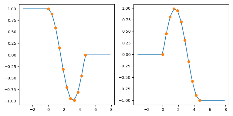
To mimic the behavior of numpy.interp with interp1d, you can use the fact that it supports a 2-tuple as the fill_value. The tuple elements are then used to fill for xnew < min(x) and x > max(x), respectively. For multidimensional y, these elements must have the same shape as y or be broadcastable to it.
To illustrate:
import numpy as np import matplotlib.pyplot as plt from scipy.interpolate import interp1d
x = np.linspace(0, 1.5*np.pi, 11) y = np.column_stack((np.cos(x), np.sin(x))) # y.shape is (11, 2)
func = interp1d(x, y, axis=0, # interpolate along columns bounds_error=False, kind='linear', fill_value=(y[0], y[-1])) xnew = np.linspace(-np.pi, 2.5*np.pi, 51) ynew = func(xnew)
fix, (ax1, ax2) = plt.subplots(1, 2, figsize=(8, 4)) ax1.plot(xnew, ynew[:, 0]) ax1.plot(x, y[:, 0], 'o')
ax2.plot(xnew, ynew[:, 1]) ax2.plot(x, y[:, 1], 'o') plt.tight_layout()
CubicSpline extend the boundary conditions#
CubicSpline needs two extra boundary conditions, which are controlled by the bc_type parameter. This parameter can either list explicit values of derivatives at the edges, or use helpful aliases. For instance, bc_type="clamped" sets the first derivatives to zero,bc_type="natural" sets the second derivatives to zero (two other recognized string values are “periodic” and “not-a-knot”)
While the extrapolation is controlled by the boundary condition, the relation is not very intuitive. For instance, one can expect that forbc_type="natural", the extrapolation is linear. This expectation is too strong: each boundary condition sets the derivatives at a single point, at the boundary only. Extrapolation is done from the first and last polynomial pieces, which — for a natural spline — is a cubic with a zero second derivative at a given point.
One other way of seeing why this expectation is too strong is to consider a dataset with only three data points, where the spline has two polynomial pieces. To extrapolate linearly, this expectation implies that both of these pieces are linear. But then, two linear pieces cannot match at a middle point with a continuous 2nd derivative! (Unless of course, if all three data points actually lie on a single straight line).
To illustrate the behavior we consider a synthetic dataset and compare several boundary conditions:
import numpy as np import matplotlib.pyplot as plt from scipy.interpolate import CubicSpline
xs = [1, 2, 3, 4, 5, 6, 7, 8] ys = [4.5, 3.6, 1.6, 0.0, -3.3, -3.1, -1.8, -1.7]
notaknot = CubicSpline(xs, ys, bc_type='not-a-knot') natural = CubicSpline(xs, ys, bc_type='natural') clamped = CubicSpline(xs, ys, bc_type='clamped') xnew = np.linspace(min(xs) - 4, max(xs) + 4, 101)
splines = [notaknot, natural, clamped] titles = ['not-a-knot', 'natural', 'clamped']
fig, axs = plt.subplots(3, 3, figsize=(12, 12)) for i in [0, 1, 2]: for j, spline, title in zip(range(3), splines, titles): axs[i, j].plot(xs, spline(xs, nu=i),'o') axs[i, j].plot(xnew, spline(xnew, nu=i),'-') axs[i, j].set_title(f'{title}, deriv={i}')
plt.tight_layout() plt.show()
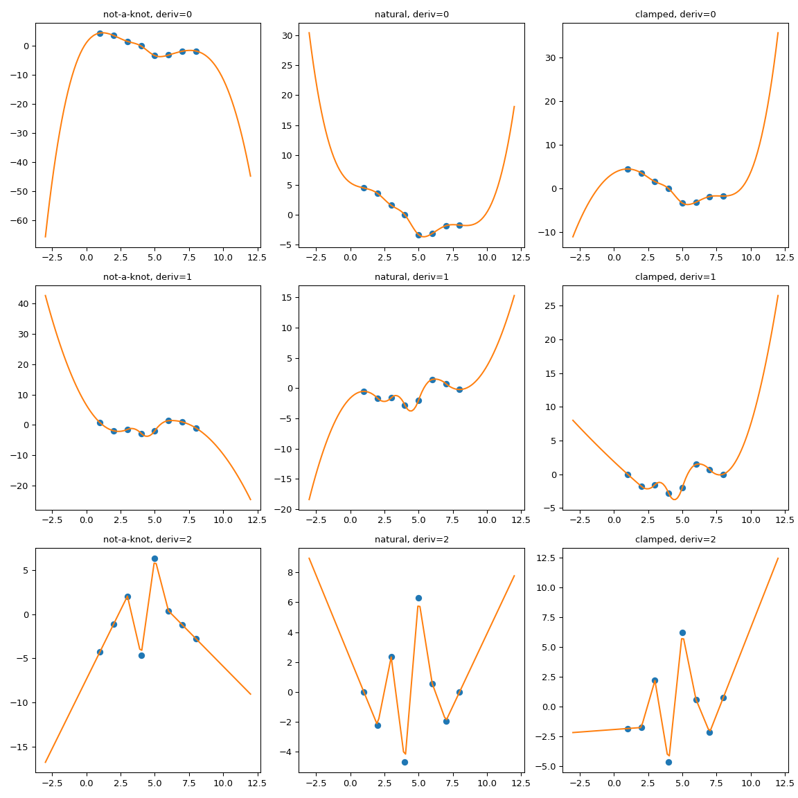
It is clearly seen that the natural spline does have the zero second derivative at the boundaries, but extrapolation is non-linear.bc_type="clamped" shows a similar behavior: first derivatives are only equal to zero exactly at the boundary. In all cases, extrapolation is done by extending the first and last polynomial pieces of the spline, whatever they happen to be.
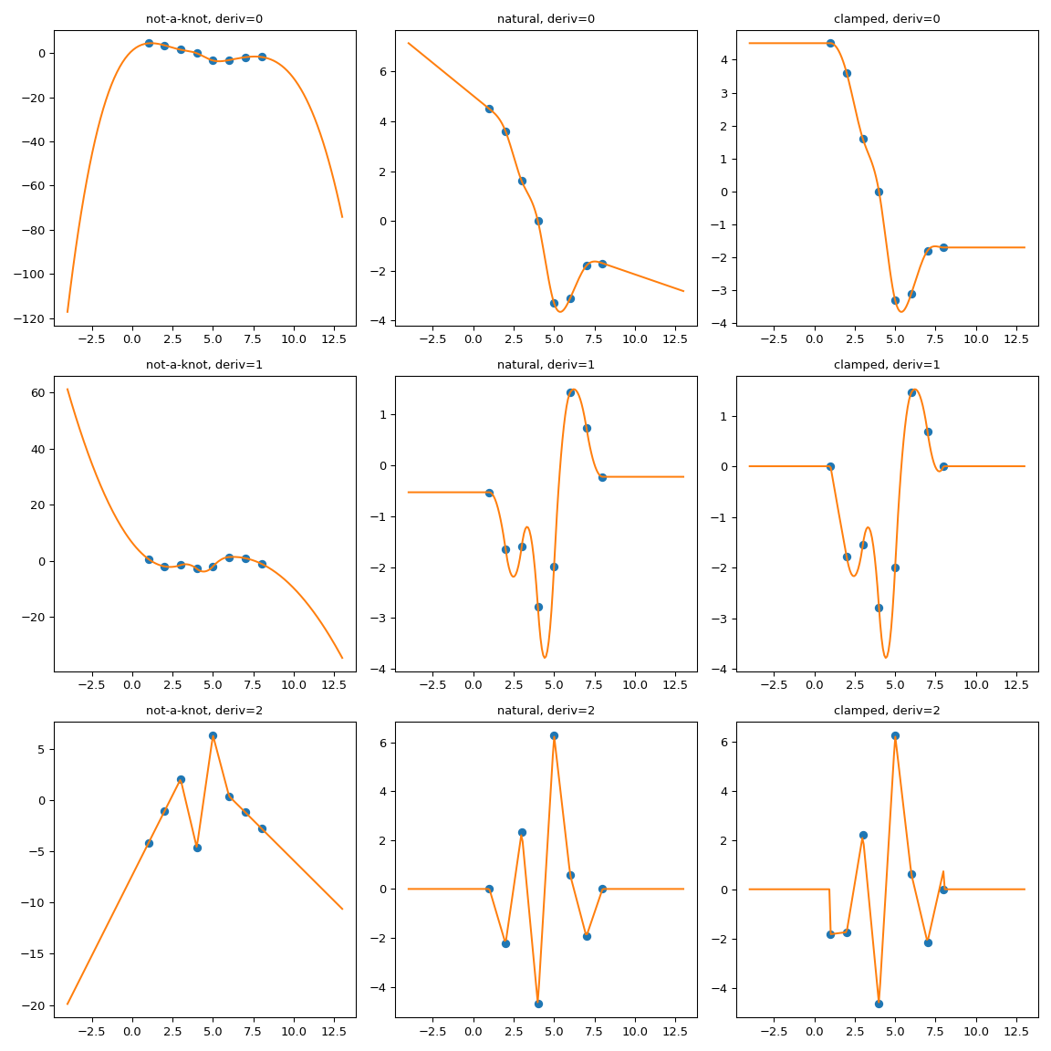
One possible way to force the extrapolation is to extend the interpolation domain to add first and last polynomial pieces which have desired properties.
Here we use extend method of the CubicSpline superclass,PPoly, to add two extra breakpoints and to make sure that the additional polynomial pieces maintain the values of the derivatives. Then the extrapolation proceeds using these two additional intervals.
import numpy as np import matplotlib.pyplot as plt from scipy.interpolate import CubicSpline
def add_boundary_knots(spline): """ Add knots infinitesimally to the left and right.
Additional intervals are added to have zero 2nd and 3rd derivatives,
and to maintain the first derivative from whatever boundary condition
was selected. The spline is modified in place.
"""
# determine the slope at the left edge
leftx = spline.x[0]
lefty = spline(leftx)
leftslope = spline(leftx, nu=1)

# add a new breakpoint just to the left and use the
# known slope to construct the PPoly coefficients.
leftxnext = np.nextafter(leftx, leftx - 1)
leftynext = lefty + leftslope*(leftxnext - leftx)
leftcoeffs = np.array([0, 0, leftslope, leftynext])
spline.extend(leftcoeffs[..., None], np.r_[leftxnext])

# repeat with additional knots to the right
rightx = spline.x[-1]
righty = spline(rightx)
rightslope = spline(rightx,nu=1)
rightxnext = np.nextafter(rightx, rightx + 1)
rightynext = righty + rightslope * (rightxnext - rightx)
rightcoeffs = np.array([0, 0, rightslope, rightynext])
spline.extend(rightcoeffs[..., None], np.r_[rightxnext])
xs = [1, 2, 3, 4, 5, 6, 7, 8] ys = [4.5, 3.6, 1.6, 0.0, -3.3, -3.1, -1.8, -1.7]
notaknot = CubicSpline(xs,ys, bc_type='not-a-knot')
not-a-knot does not require additional intervals
natural = CubicSpline(xs,ys, bc_type='natural')
extend the natural natural spline with linear extrapolating knots
add_boundary_knots(natural)
clamped = CubicSpline(xs,ys, bc_type='clamped')
extend the clamped spline with constant extrapolating knots
add_boundary_knots(clamped)
xnew = np.linspace(min(xs) - 5, max(xs) + 5, 201)
fig, axs = plt.subplots(3, 3,figsize=(12,12))
splines = [notaknot, natural, clamped] titles = ['not-a-knot', 'natural', 'clamped']
for i in [0, 1, 2]: for j, spline, title in zip(range(3), splines, titles): axs[i, j].plot(xs, spline(xs, nu=i),'o') axs[i, j].plot(xnew, spline(xnew, nu=i),'-') axs[i, j].set_title(f'{title}, deriv={i}')
plt.tight_layout() plt.show()
Manually implement the asymptotics#
The previous trick of extending the interpolation domain relies on theCubicSpline.extend method. A somewhat more general alternative is to implement a wrapper which handles the out-of-bounds behavior explicitly. Let us consider a worked example.
The setup#
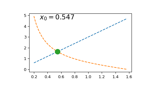
Suppose we want to solve at a given value of \(a\) the equation
\[a x = 1/\tan{x}\;.\]
(One application where these kinds of equations appear is solving for energy levels of a quantum particle). For simplicity, let’s only consider \(x\in (0, \pi/2)\).
Solving this equation once is straightforward:
import numpy as np import matplotlib.pyplot as plt from scipy.optimize import brentq
def f(x, a): return a*x - 1/np.tan(x)
a = 3 x0 = brentq(f, 1e-16, np.pi/2, args=(a,)) # here we shift the left edge # by a machine epsilon to avoid # a division by zero at x=0 xx = np.linspace(0.2, np.pi/2, 101) plt.plot(xx, axx, '--') plt.plot(xx, 1/np.tan(xx), '--') plt.plot(x0, ax0, 'o', ms=12) plt.text(0.1, 0.9, fr'$x_0 = {x0:.3f}$', transform=plt.gca().transAxes, fontsize=16) plt.show()
However, if we need to solve it multiple times (e.g. to find _a series_of roots due to periodicity of the tan function), repeated calls toscipy.optimize.brentq become prohibitively expensive.
To circumvent this difficulty, we tabulate \(y = ax - 1/\tan{x}\)and interpolate it on the tabulated grid. In fact, we will use the _inverse_interpolation: we interpolate the values of \(x\) versus \(у\). This way, solving the original equation becomes simply an evaluation of the interpolated function at zero \(y\) argument.
To improve the interpolation accuracy we will use the knowledge of the derivatives of the tabulated function. We will useBPoly.from_derivatives to construct a cubic interpolant (equivalently, we could have used CubicHermiteSpline)
import numpy as np import matplotlib.pyplot as plt from scipy.interpolate import BPoly
def f(x, a): return a*x - 1/np.tan(x)
xleft, xright = 0.2, np.pi/2 x = np.linspace(xleft, xright, 11)
fig, ax = plt.subplots(1, 2, figsize=(12, 4))
for j, a in enumerate([3, 93]): y = f(x, a) dydx = a + 1./np.sin(x)**2 # d(ax - 1/tan(x)) / dx dxdy = 1 / dydx # dx/dy = 1 / (dy/dx)
xdx = np.c_[x, dxdy]
spl = BPoly.from_derivatives(y, xdx)   # inverse interpolation

yy = np.linspace(f(xleft, a), f(xright, a), 51)
ax[j].plot(yy, spl(yy), '--')
ax[j].plot(y, x, 'o')
ax[j].set_xlabel(r'$y$')
ax[j].set_ylabel(r'$x$')
ax[j].set_title(rf'$a = {a}$')

ax[j].plot(0, spl(0), 'o', ms=12)
ax[j].text(0.1, 0.85, fr'$x_0 = {spl(0):.3f}$',
           transform=ax[j].transAxes, fontsize=18)
ax[j].grid(True)
plt.tight_layout() plt.show()
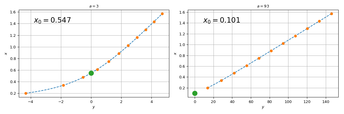
Note that for \(a=3\), spl(0) agrees with the brentq call above, while for \(a = 93\), the difference is substantial. The reason the procedure starts failing for large \(a\) is that the straight line \(y = ax\) tends towards the vertical axis, and the root of the original equation tends towards \(x=0\). Since we tabulated the original function at a finite grid, spl(0) involves extrapolation for too-large values of \(a\). Relying on extrapolation is prone to losing accuracy and is best avoided.
Use the known asymptotics#
Looking at the original equation, we note that for \(x\to 0\),\(\tan(x) = x + O(x^3)\), and the original equation becomes
\[ax = 1/x \;,\]
so that \(x_0 \approx 1/\sqrt{a}\) for \(a \gg 1\).
We will use this to cook up a class which switches from interpolation to using this known asymptotic behavior for out-of-range data. A bare-bones implementation may look like this
class RootWithAsymptotics: def init(self, a):
   # construct the interpolant
   xleft, xright = 0.2, np.pi/2
   x = np.linspace(xleft, xright, 11)

   y = f(x, a)
   dydx = a + 1./np.sin(x)**2    # d(ax - 1/tan(x)) / dx
   dxdy = 1 / dydx               # dx/dy = 1 / (dy/dx)

   # inverse interpolation
   self.spl = BPoly.from_derivatives(y, np.c_[x, dxdy])
   self.a = a
def root(self): out = self.spl(0) asympt = 1./np.sqrt(self.a) return np.where(spl.x.min() < asympt, out, asympt)
And then
r = RootWithAsymptotics(93) r.root() array(0.10369517)
which differs from the extrapolated result and agrees with the brentq call.
Note that this implementation is intentionally pared down. From the API perspective, you may want to instead implement the __call__ method so that the full dependence of x on y is available. From the numerical perspective, more work is needed to make sure that the switch between interpolation and asymptotics occurs deep enough into the asymptotic regime, so that the resulting function is smooth enough at the switch-over point.
Also in this example we artificially limited the problem to only consider a single periodicity interval of the tan function, and only dealt with \(a > 0\). For negative values of \(a\), we would need to implement the other asymptotics, for \(x\to \pi\).
However the basic idea is the same.