tfqmr - Solve system of linear equations — transpose-free quasi-minimal residual
method - MATLAB ([original](https://in.mathworks.com/help/matlab/ref/tfqmr.html)) ([raw](?raw))Solve system of linear equations — transpose-free quasi-minimal residual method
Syntax
Description
[x](#br02iz4-1%5Fsep%5Fmw%5Fb2afce71-ce1a-494a-85e3-71dd5f36e7d7) = tfqmr([A](#mw%5F698b2328-a822-4165-b90e-3b426eead0a5),[b](#br02iz4-1%5Fsep%5Fmw%5F3800dea9-6306-44ef-9490-f16e20ceb7ab)) attempts to solve the system of linear equations A*x = b forx using the Transpose-free Quasi-minimal Residual Method. When the attempt is successful, tfqmr displays a message to confirm convergence. Iftfqmr fails to converge after the maximum number of iterations or halts for any reason, it displays a diagnostic message that includes the relative residualnorm(b-A*x)/norm(b) and the iteration number at which the method stopped.
[x](#br02iz4-1%5Fsep%5Fmw%5Fb2afce71-ce1a-494a-85e3-71dd5f36e7d7) = tfqmr([A](#mw%5F698b2328-a822-4165-b90e-3b426eead0a5),[b](#br02iz4-1%5Fsep%5Fmw%5F3800dea9-6306-44ef-9490-f16e20ceb7ab),[tol](#br02iz4-1%5Fsep%5Fmw%5Fb797b123-ccd8-4b99-a496-07d543d1a21b)) specifies a tolerance for the method. The default tolerance is1e-6.
[x](#br02iz4-1%5Fsep%5Fmw%5Fb2afce71-ce1a-494a-85e3-71dd5f36e7d7) = tfqmr([A](#mw%5F698b2328-a822-4165-b90e-3b426eead0a5),[b](#br02iz4-1%5Fsep%5Fmw%5F3800dea9-6306-44ef-9490-f16e20ceb7ab),[tol](#br02iz4-1%5Fsep%5Fmw%5Fb797b123-ccd8-4b99-a496-07d543d1a21b),[maxit](#br02iz4-1%5Fsep%5Fmw%5F843917a7-f520-49f0-8815-7ffb3f307a16)) specifies the maximum number of iterations to use. tfqmr displays a diagnostic message if it fails to converge within maxit iterations.
[x](#br02iz4-1%5Fsep%5Fmw%5Fb2afce71-ce1a-494a-85e3-71dd5f36e7d7) = tfqmr([A](#mw%5F698b2328-a822-4165-b90e-3b426eead0a5),[b](#br02iz4-1%5Fsep%5Fmw%5F3800dea9-6306-44ef-9490-f16e20ceb7ab),[tol](#br02iz4-1%5Fsep%5Fmw%5Fb797b123-ccd8-4b99-a496-07d543d1a21b),[maxit](#br02iz4-1%5Fsep%5Fmw%5F843917a7-f520-49f0-8815-7ffb3f307a16),[M](#br02iz4-1%5Fsep%5Fmw%5Fa88cd7b1-4dcd-46dd-8611-81acb80fe667)) specifies a preconditioner matrix M and computes x by effectively solving the system AM−1y=b for y, where y=Mx. Using a preconditioner matrix can improve the numerical properties of the problem and the efficiency of the calculation.
[x](#br02iz4-1%5Fsep%5Fmw%5Fb2afce71-ce1a-494a-85e3-71dd5f36e7d7) = tfqmr([A](#mw%5F698b2328-a822-4165-b90e-3b426eead0a5),[b](#br02iz4-1%5Fsep%5Fmw%5F3800dea9-6306-44ef-9490-f16e20ceb7ab),[tol](#br02iz4-1%5Fsep%5Fmw%5Fb797b123-ccd8-4b99-a496-07d543d1a21b),[maxit](#br02iz4-1%5Fsep%5Fmw%5F843917a7-f520-49f0-8815-7ffb3f307a16),[M1](#br02iz4-1%5Fsep%5Fmw%5Fa88cd7b1-4dcd-46dd-8611-81acb80fe667),[M2](#br02iz4-1%5Fsep%5Fmw%5Fa88cd7b1-4dcd-46dd-8611-81acb80fe667)) specifies factors of the preconditioner matrix M such that M = M1*M2.
[x](#br02iz4-1%5Fsep%5Fmw%5Fb2afce71-ce1a-494a-85e3-71dd5f36e7d7) = tfqmr([A](#mw%5F698b2328-a822-4165-b90e-3b426eead0a5),[b](#br02iz4-1%5Fsep%5Fmw%5F3800dea9-6306-44ef-9490-f16e20ceb7ab),[tol](#br02iz4-1%5Fsep%5Fmw%5Fb797b123-ccd8-4b99-a496-07d543d1a21b),[maxit](#br02iz4-1%5Fsep%5Fmw%5F843917a7-f520-49f0-8815-7ffb3f307a16),[M1](#br02iz4-1%5Fsep%5Fmw%5Fa88cd7b1-4dcd-46dd-8611-81acb80fe667),[M2](#br02iz4-1%5Fsep%5Fmw%5Fa88cd7b1-4dcd-46dd-8611-81acb80fe667),[x0](#br02iz4-1%5Fsep%5Fmw%5F40e27791-2264-4d42-8cb6-b8bf869783bc)) specifies an initial guess for the solution vector x. The default is a vector of zeros.
[[x](#br02iz4-1%5Fsep%5Fmw%5Fb2afce71-ce1a-494a-85e3-71dd5f36e7d7),[flag](#br02iz4-1%5Fsep%5Fmw%5F1f278699-812f-4628-8d99-e8f6ae362e34)] = tfqmr(___) returns a flag that specifies whether the algorithm successfully converged. Whenflag = 0, convergence was successful. You can use this output syntax with any of the previous input argument combinations. When you specify theflag output, tfqmr does not display any diagnostic messages.
[[x](#br02iz4-1%5Fsep%5Fmw%5Fb2afce71-ce1a-494a-85e3-71dd5f36e7d7),[flag](#br02iz4-1%5Fsep%5Fmw%5F1f278699-812f-4628-8d99-e8f6ae362e34),[relres](#br02iz4-1%5Fsep%5Fmw%5F6de229ba-091b-4137-acf4-6c7691a0398c)] = tfqmr(___) also returns the relative residual norm(b-A*x)/norm(b). Ifflag is 0, then relres <= tol.
[[x](#br02iz4-1%5Fsep%5Fmw%5Fb2afce71-ce1a-494a-85e3-71dd5f36e7d7),[flag](#br02iz4-1%5Fsep%5Fmw%5F1f278699-812f-4628-8d99-e8f6ae362e34),[relres](#br02iz4-1%5Fsep%5Fmw%5F6de229ba-091b-4137-acf4-6c7691a0398c),[iter](#mw%5Fc22b4c51-edd7-4050-955b-85a815b7cba5)] = tfqmr(___) also returns the iteration number iter at which x was computed.
[[x](#br02iz4-1%5Fsep%5Fmw%5Fb2afce71-ce1a-494a-85e3-71dd5f36e7d7),[flag](#br02iz4-1%5Fsep%5Fmw%5F1f278699-812f-4628-8d99-e8f6ae362e34),[relres](#br02iz4-1%5Fsep%5Fmw%5F6de229ba-091b-4137-acf4-6c7691a0398c),[iter](#mw%5Fc22b4c51-edd7-4050-955b-85a815b7cba5),[resvec](#mw%5F94617f4c-5926-405d-b3a9-c02801a6ca08)] = tfqmr(___) also returns a vector of the residual norm at each half iteration, including the first residual norm(b-A*x0).
Examples
Solve a square linear system using tfqmr with default settings, and then adjust the tolerance and number of iterations used in the solution process.
Create a random sparse matrix A with 50% density. Also create a random vector b for the right-hand side of Ax=b.
rng default A = sprand(400,400,.5); A = A'*A; b = rand(400,1);
Solve Ax=b using tfqmr. The output display includes the value of the relative residual error ‖b-Ax‖‖b‖.
tfqmr stopped at iteration 40 without converging to the desired tolerance 1e-06 because the maximum number of iterations was reached. The iterate returned (number 13) has relative residual 0.29.
By default tfqmr uses 40 iterations and a tolerance of 1e-6, and the algorithm is unable to converge in those 40 iterations for this matrix. Since the residual is still large, it is a good indicator that more iterations (or a preconditioner matrix) are needed. You also can use a larger tolerance to make it easier for the algorithm to converge.
Solve the system again using a tolerance of 1e-4 and 100 iterations.
tfqmr stopped at iteration 200 without converging to the desired tolerance 0.0001 because the maximum number of iterations was reached. The iterate returned (number 13) has relative residual 0.29.
Even with a looser tolerance and more iterations the residual error does not improve much. When an iterative algorithm stalls in this manner it is a good indication that a preconditioner matrix is needed.
Calculate the incomplete Cholesky factorization of A, and use the L' factor as a preconditioner input to tfqmr.
L = ichol(A); x = tfqmr(A,b,1e-4,100,L');
tfqmr converged at iteration 32 to a solution with relative residual 4.2e-05.
Using a preconditioner improves the numerical properties of the problem enough that tfqmr is able to converge.
Examine the effect of using a preconditioner matrix with tfqmr to solve a linear system.
Load west0479, a real 479-by-479 nonsymmetric sparse matrix.
load west0479 A = west0479;
Define b so that the true solution to Ax=b is a vector of all ones.
Set the tolerance and maximum number of iterations.
Use tfqmr to find a solution at the requested tolerance and number of iterations. Specify five outputs to return information about the solution process:
xis the computed solution toA*x = b.fl0is a flag indicating whether the algorithm converged.rr0is the relative residual of the computed answerx.it0is the iteration number whenxwas computed.rv0is a vector of the residual history for ‖b-Ax‖.
[x,fl0,rr0,it0,rv0] = tfqmr(A,b,tol,maxit); fl0
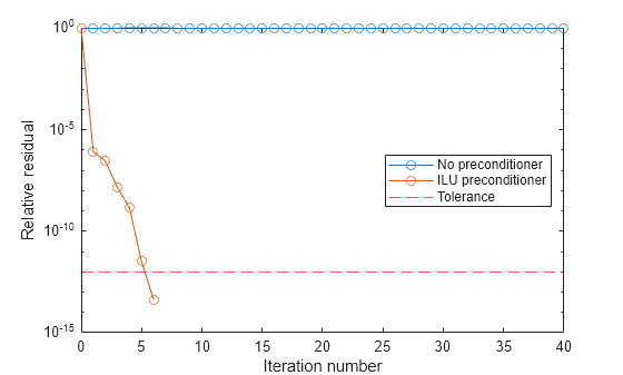
fl0 is 1 because tfqmr does not converge to the requested tolerance 1e-12 within the requested 20 iterations. The tenth iterate is the best approximate solution and is the one returned as indicated by it0 = 10.
To aid with the slow convergence, you can specify a preconditioner matrix. Since A is nonsymmetric, use ilu to generate the preconditioner M=L U. Specify a drop tolerance to ignore nondiagonal entries with values smaller than 1e-6. Solve the preconditioned system A M-1M x=b by specifying L and U as inputs to tfqmr.
setup = struct('type','ilutp','droptol',1e-6); [L,U] = ilu(A,setup); [x1,fl1,rr1,it1,rv1] = tfqmr(A,b,tol,maxit,L,U); fl1
The use of an ilu preconditioner produces a relative residual less than the prescribed tolerance of 1e-12 at the third iteration. The output rv1(1) is norm(b), and the output rv1(end) is norm(b-A*x1).
You can follow the progress of tfqmr by plotting the relative residuals at each iteration. Plot the residual history of each solution with a line for the specified tolerance. Note that like bicgstab, tfqmr tracks half iterations.
semilogy(0:length(rv0)-1,rv0/norm(b),'-o') hold on semilogy(0:length(rv1)-1,rv1/norm(b),'-o') yline(tol,'r--'); legend('No preconditioner','ILU preconditioner','Tolerance','Location','East') xlabel('Iteration number') ylabel('Relative residual')
Examine the effect of supplying tfqmr with an initial guess of the solution.
Create a tridiagonal sparse matrix. Use the sum of each row as the vector for the right-hand side of Ax=b so that the expected solution for x is a vector of ones.
n = 900; e = ones(n,1); A = spdiags([e 2*e e],-1:1,n,n); b = sum(A,2);
Use tfqmr to solve Ax=b twice: one time with the default initial guess, and one time with a good initial guess of the solution. Use 200 iterations and the default tolerance for both solutions. Specify the initial guess in the second solution as a vector with all elements equal to 0.99.
maxit = 200; x1 = tfqmr(A,b,[],maxit);
tfqmr converged at iteration 19 to a solution with relative residual 9.6e-07.
x0 = 0.99*e; x2 = tfqmr(A,b,[],maxit,[],[],x0);
tfqmr converged at iteration 4 to a solution with relative residual 7.9e-07.
In this case supplying an initial guess enables tfqmr to converge more quickly.
Returning Intermediate Results
You also can use the initial guess to get intermediate results by calling tfqmr in a for-loop. Each call to the solver performs a few iterations and stores the calculated solution. Then you use that solution as the initial vector for the next batch of iterations.
For example, this code performs 100 iterations four times and stores the solution vector after each pass in the for-loop:
x0 = zeros(size(A,2),1); tol = 1e-8; maxit = 100; for k = 1:4 [x,flag,relres] = tfqmr(A,b,tol,maxit,[],[],x0); X(:,k) = x; R(k) = relres; x0 = x; end
X(:,k) is the solution vector computed at iteration k of the for-loop, and R(k) is the relative residual of that solution.
Solve a linear system by providing tfqmr with a function handle that computes A*x in place of the coefficient matrix A.
One of the Wilkinson test matrices generated by gallery is a 21-by-21 tridiagonal matrix. Preview the matrix.
A = 21×21
10     1     0     0     0     0     0     0     0     0     0     0     0     0     0     0     0     0     0     0     0
 1     9     1     0     0     0     0     0     0     0     0     0     0     0     0     0     0     0     0     0     0
 0     1     8     1     0     0     0     0     0     0     0     0     0     0     0     0     0     0     0     0     0
 0     0     1     7     1     0     0     0     0     0     0     0     0     0     0     0     0     0     0     0     0
 0     0     0     1     6     1     0     0     0     0     0     0     0     0     0     0     0     0     0     0     0
 0     0     0     0     1     5     1     0     0     0     0     0     0     0     0     0     0     0     0     0     0
 0     0     0     0     0     1     4     1     0     0     0     0     0     0     0     0     0     0     0     0     0
 0     0     0     0     0     0     1     3     1     0     0     0     0     0     0     0     0     0     0     0     0
 0     0     0     0     0     0     0     1     2     1     0     0     0     0     0     0     0     0     0     0     0
 0     0     0     0     0     0     0     0     1     1     1     0     0     0     0     0     0     0     0     0     0
 0     0     0     0     0     0     0     0     0     1     0     1     0     0     0     0     0     0     0     0     0
 0     0     0     0     0     0     0     0     0     0     1     1     1     0     0     0     0     0     0     0     0
 0     0     0     0     0     0     0     0     0     0     0     1     2     1     0     0     0     0     0     0     0
 0     0     0     0     0     0     0     0     0     0     0     0     1     3     1     0     0     0     0     0     0
 0     0     0     0     0     0     0     0     0     0     0     0     0     1     4     1     0     0     0     0     0
  ⋮
The Wilkinson matrix has a special structure, so you can represent the operation A*x with a function handle. When A multiplies a vector, most of the elements in the resulting vector are zeros. The nonzero elements in the result correspond with the nonzero tridiagonal elements of A. Moreover, only the main diagonal has nonzeros that are not equal to 1.
The expression Ax becomes:
Ax=[1010⋯⋯⋯001910001810⋮⋮0171001610⋮⋮0151001410⋮⋮013⋱000⋱⋱100⋯⋯⋯0110][x1x2x3x4x5⋮⋮x21]=[10x1+x2x1+9x2+x3x2+8x3+x4⋮x19+9x20+x21x20+10x21].
The resulting vector can be written as the sum of three vectors:
Ax=[0+10x1+x2x1+9x2+x3x2+8x3+x4⋮x19+9x20+x21x20+10x21+0]=[0x1⋮x20]+[10x19x2⋮10x21]+[x2⋮x210].
In MATLAB®, write a function that creates these vectors and adds them together, thus giving the value of A*x:
function y = afun(x) y = [0; x(1:20)] + ... [(10:-1:0)'; (1:10)'].*x + ... [x(2:21); 0]; end
(This function is saved as a local function at the end of the example.)
Now, solve the linear system Ax=b by providing tfqmr with the function handle that calculates A*x. Use a tolerance of 1e-12 and 50 iterations.
b = ones(21,1);
tol = 1e-12;
maxit = 50;
x1 = tfqmr(@afun,b,tol,maxit)
tfqmr converged at iteration 10 to a solution with relative residual 6.7e-15.
x1 = 21×1
0.0910
0.0899
0.0999
0.1109
0.1241
0.1443
0.1544
0.2383
0.1309
0.5000
0.3691
0.5000
0.1309
0.2383
0.1544
  ⋮
Check that afun(x1) produces a vector of ones.
ans = 21×1
1.0000
1.0000
1.0000
1.0000
1.0000
1.0000
1.0000
1.0000
1.0000
1.0000
1.0000
1.0000
1.0000
1.0000
1.0000
  ⋮
Local Functions
function y = afun(x) y = [0; x(1:20)] + ... [(10:-1:0)'; (1:10)'].*x + ... [x(2:21); 0]; end
Input Arguments
Coefficient matrix, specified as a square matrix or function handle. This matrix is the coefficient matrix in the linear system A*x = b. Generally,A is a large sparse matrix or a function handle that returns the product of a large sparse matrix and column vector.
Specifying A as a Function Handle
You can optionally specify the coefficient matrix as a function handle instead of a matrix. The function handle returns matrix-vector products instead of forming the entire coefficient matrix, making the calculation more efficient.
To use a function handle, use the function signature function y = afun(x). Parameterizing Functions explains how to provide additional parameters to the function afun, if necessary. The function call afun(x) must return the value of A*x.
Data Types: single | double | function_handle
Complex Number Support: Yes
Right side of linear equation, specified as a column vector. The length of b must be equal tosize(A,1).
Data Types: single | double
Complex Number Support: Yes
Method tolerance, specified as a positive scalar. Use this input to trade off accuracy and runtime in the calculation. tfqmr must meet the tolerance within the number of allowed iterations to be successful. A smaller value of tol means the answer must be more precise for the calculation to be successful.
Data Types: single | double
Maximum number of iterations, specified as a positive scalar integer. Increase the value ofmaxit to allow more iterations fortfqmr to meet the tolerance tol. Generally, a smaller value of tol means more iterations are required to successfully complete the calculation.
Data Types: single | double
Preconditioner matrices, specified as separate arguments of matrices or function handles. You can specify a preconditioner matrix M or its matrix factors M = M1*M2 to improve the numerical aspects of the linear system and make it easier for tfqmr to converge quickly. You can use the incomplete matrix factorization functions ilu and ichol to generate preconditioner matrices. You also can use equilibrate prior to factorization to improve the condition number of the coefficient matrix. For more information on preconditioners, see Iterative Methods for Linear Systems.
tfqmr treats unspecified preconditioners as identity matrices.
Specifying M as a Function Handle
You can optionally specify any of M, M1, orM2 as function handles instead of matrices. The function handle performs matrix-vector operations instead of forming the entire preconditioner matrix, making the calculation more efficient.
To use a function handle, use the function signature function y = mfun(x). Parameterizing Functions explains how to provide additional parameters to the function mfun, if necessary. The function call mfun(x) must return the value ofM\x or M2\(M1\x).
Data Types: single | double | function_handle
Complex Number Support: Yes
Initial guess, specified as a column vector with length equal to size(A,2). If you can provide tfqmr with a more reasonable initial guessx0 than the default vector of zeros, then it can save computation time and help the algorithm converge faster.
Data Types: single | double
Complex Number Support: Yes
Output Arguments
Linear system solution, returned as a column vector. This output gives the approximate solution to the linear system A*x = b. If the calculation is successful (flag = 0), then relres is less than or equal to tol.
Whenever the calculation is not successful (flag ~= 0), the solutionx returned by tfqmr is the one with minimal residual norm computed over all the iterations.
Data Types: single | double
Convergence flag, returned as one of the scalar values in this table. The convergence flag indicates whether the calculation was successful and differentiates between several different forms of failure.
| Flag Value | Convergence |
|---|---|
| 0 | Success — tfqmr converged to the desired tolerance tol withinmaxit iterations. |
| 1 | Failure — tfqmr iteratedmaxit iterations but did not converge. |
| 2 | Failure — The preconditioner matrix M orM = M1*M2 is ill conditioned. |
| 3 | Failure — tfqmr stagnated after two consecutive iterations were the same. |
| 4 | Failure — One of the scalar quantities calculated by thetfqmr algorithm became too small or too large to continue computing. |
Relative residual error, returned as a scalar. The relative residual error relres = norm(b-A*x)/norm(b) is an indication of how accurate the answer is. If the calculation converges to the tolerance tol within maxit iterations, then relres <= tol.
Data Types: single | double
Iteration number, returned as a scalar. This output indicates the iteration number at which the computed answer for x was calculated. Each outer iteration of tfqmr includes two inner iterations, soiter can be returned as a decimal number of iterations.
Data Types: double
Residual error, returned as a vector. The residual errornorm(b-A*x) reveals how close the algorithm is to converging for a given value of x. The number of elements in resvec is equal to the number of half iterations. You can examine the contents ofresvec to help decide whether to change the values oftol or maxit.
Data Types: single | double
More About
Just as the CGS method was developed to avoid the use of the transpose of the coefficient matrix in BiCG, the TFQMR method was developed to avoid the use of the transpose in QMR. These "squared" methods require an extra matrix-vector product per step compared to the "unsquared" versions (BiCG and QMR), so they are slightly less efficient.
The TFQMR method is on-par with CGS, but has much smoother convergence. Still, since TFQMR ultimately uses the BiCG polynomial, it breaks down whenever CGS does [1].
Tips
- Convergence of most iterative methods depends on the condition number of the coefficient matrix,
cond(A). WhenAis square, you can use equilibrate to improve its condition number, and on its own this makes it easier for most iterative solvers to converge. However, usingequilibratealso leads to better quality preconditioner matrices when you subsequently factor the equilibrated matrixB = R*P*A*C. - You can use matrix reordering functions such as
dissectandsymrcmto permute the rows and columns of the coefficient matrix and minimize the number of nonzeros when the coefficient matrix is factored to generate a preconditioner. This can reduce the memory and time required to subsequently solve the preconditioned linear system.
References
[1] Barrett, R., M. Berry, T. F. Chan, et al., Templates for the Solution of Linear Systems: Building Blocks for Iterative Methods, SIAM, Philadelphia, 1994.
Extended Capabilities
The tfqmr function supports GPU array input with these usage notes and limitations:
- When input
Ais a sparse matrix:- If you use two preconditioners,
M1andM2, then they must be lower triangular and upper triangular matrices, or both of them must be function handles. Using lower triangular and upper triangular preconditioner matrices instead of function handles can significantly improve computation speed. - For GPU arrays,
tfqmrdoes not detect stagnation (Flag 3). Instead, it reports failure to converge (Flag 1).
- If you use two preconditioners,
For more information, see Run MATLAB Functions on a GPU (Parallel Computing Toolbox).
Version History
Introduced before R2006a
You can specify these arguments as single precision:
A— Coefficient matrixb— Right side of linear equationM,M1,M2— Preconditioner matricesx0— Initial guess
If you specify any of these arguments as single precision, the function computes in single precision and returns the linear system solution, relative residual error, and residual error outputs as type single. For faster computation, specify all arguments, including function handle outputs, as the same precision.