istftLayer - Inverse short-time Fourier transform layer - MATLAB (original) (raw)
Inverse short-time Fourier transform layer
Since R2024a
Description
An ISTFT layer computes the inverse short-time Fourier transform of the input. Use of this layer requires Deep Learning Toolbox™.
Creation
Syntax
Description
`layer` = istftLayer creates an Inverse Short-Time Fourier Transform (ISTFT) layer. The input to istftLayer must be a real-valued dlarray (Deep Learning Toolbox) object in"CBT" or "SCBT" format.
- For
"CBT"inputs, the size of the channel ("C") dimension must be even and divisible byfloor(`FFTLength`/2)+1. - For
"SCBT"inputs, the size of the spatial ("S") dimension must equalfloor(`FFTLength`/2)+1.
The output of istftLayer is a real-valued array in"CBT" format. For more information, see Layer Input and Output Formats.
Note
When you initialize the learnable parameters of istftLayer, the layer weights are set to the synthesis window used to compute the transform. It is not recommended to initialize the weights directly.
`layer` = istftLayer([PropertyName=Value](#mw%5F24aa14e6-d641-4d9a-b79c-a6e74ed66858)) creates an ISTFT layer with properties specified by one or more name-value arguments. You can specify the analysis window and the number of overlapped samples, among others.
Note
You cannot use this syntax to set the Weights property.
Properties
ISTFT
This property is read-only.
Windowing function used to compute the ISTFT, specified as a vector with two or more elements. For perfect reconstruction, use the same window as in stftLayer.
For a list of available windows, see Windows.
You can set this property when you create an istftLayer object. After you create an istftLayer object, this property is read-only.
Example: hann(N+1) and(1-cos(2*pi*(0:N)'/N))/2 both specify a Hann window of lengthN + 1.
Data Types: double | single
This property is read-only.
Number of overlapped samples, specified as a nonnegative integer smaller than the length of window. If you omit OverlapLength or specify it as empty, the object sets it to the largest integer less than 75% of the window length, which turns out to be 96 samples for the default Hann window. Equivalently, the stride between adjoining segments is 32 samples.
You can set this property when you create an istftLayer object. After you create an istftLayer object, this property is read-only.
Data Types: double | single
This property is read-only.
Number of discrete Fourier transform (DFT) points, specified as a positive integer greater than or equal to the window length. To achieve perfect time-domain reconstruction, set the number of DFT points to match that used in stftLayer.
You can set this property when you create an istftLayer object. After you create an istftLayer object, this property is read-only.
Data Types: double | single
This property is read-only.
Method of overlap-add, specified as one of these:
"wola"— Weighted overlap-add"ola"— Overlap-add
You can set this property when you create an istftLayer object. After you create an istftLayer object, this property is read-only.
This property is read-only.
Expected number of channels and samples output by istftLayer, specified as a two-element vector of positive integers. The first element is the expected number of channels, and the second element is the expected number of time samples.
By default, istftLayer does not check the output size of the ISTFT. If you specify ExpectedOutputSize,istftLayer errors if the inverse short-time Fourier transform for the given inputs do not match ExpectedOutputSize in the number of channels and samples.
You can set this property when you create an istftLayer object. After you create an istftLayer object, this property is read-only.
Data Types: single | double
Layer
Layer weights, specified as [], a numeric array, or adlarray object.
The layer weights are learnable parameters. You can use initialize (Deep Learning Toolbox) to initialize the learnable parameters of a dlnetwork (Deep Learning Toolbox) that includesistftLayer objects. When you initialize the layers,initialize sets Weights to the synthesis window used to compute the transform. For more information, see Initialize Inverse Short-Time Fourier Transform Layer.. (since R2025a)
It is not recommended to initialize the weights directly.
Data Types: double | single
Multiplier for weight learning rate, specified as a nonnegative scalar. If you do not specify this property, it defaults to zero, resulting in weights that do not update with training. You can also set this property using the setLearnRateFactor (Deep Learning Toolbox) function.
Data Types: double | single
Data Types: char | string
This property is read-only.
Number of inputs to the layer, stored as 1. This layer accepts a single input only.
Data Types: double
This property is read-only.
Input names, stored as {'in'}. This layer accepts a single input only.
Data Types: cell
This property is read-only.
Number of outputs from the layer, stored as 1. This layer has a single output only.
Data Types: double
This property is read-only.
Output names, stored as {'out'}. This layer has a single output only.
Data Types: cell
Examples
Create an inverse short-time Fourier transform layer. Specify a 64-sample Hamming window. Specify 63 overlapped samples between adjoining segments.
layer = istftLayer(Window=hamming(64),OverlapLength=63)
layer = istftLayer with properties:
                 Name: ''
WeightLearnRateFactor: 0
               Window: [64×1 double]
        OverlapLength: 63
            FFTLength: 64
               Method: 'wola'
   ExpectedOutputSize: 'none'
Learnable Parameters Weights: []
State Parameters No properties.
Show all properties
Create an array of five layers, containing a sequence input layer, an STFT layer, an LSTM layer, an ISTFT layer, and a regression layer. There is one feature in the sequence input. Set the minimum signal length in the sequence input layer to 2048 samples. Use the default window of length 128 for both STFT and ISTFT layers.
layers = [ sequenceInputLayer(1,MinLength=2048) stftLayer(TransformMode="realimag") lstmLayer(130) fullyConnectedLayer(130) istftLayer];
Create a random array containing a batch of 10 signals and 2048 samples. Save the signal as a dlarray in "CBT" format. Analyze the layers as a dlnetwork using the example network input.
networkInput = dlarray(randn(1,10,2048,"single"),"CBT"); analyzeNetwork(layers,networkInput,targetusage="dlnetwork")

Create a deep learning network that demonstrates perfect reconstruction of the short-time Fourier transform (STFT) of a dlarray. To minimize edge effects, the network zero-pads the data before computing the STFT.
Generate a 3-by-2000-by-5 array containing five batches of a three-channel sinusoidal signal sampled at 1 kHz for two seconds. Save the array as a dlarray, specifying the dimensions in order. dlarray permutes the array dimensions to the "CBT" shape expected by a deep learning network. Display the array dimension sizes.
Fs = 1e3; nchan = 3; nbtch = 5; nsamp = 2000; t = (0:nsamp-1)/Fs;
x = zeros(nchan,nsamp,nbtch); for k=1:nbtch x(:,:,k) = sin(kpi.(1:nchan)'t)+cos(kpi.*(1:nchan)'*t); end
xd = dlarray(x,"CTB");
Design a periodic Hann window of length 100 and set the number of overlap samples to 75. Check the window and overlap length for COLA compliance.
nwin = 100; win = hann(nwin,"periodic"); noverlap = 75;
tf = iscola(win,noverlap)
Create a STFT layer that uses the Hann window. Set the number of overlap samples to 75 and FFT length to 128. Set the layer transform mode to "realimag" to concatenate the real and imaginary parts of the layer output along the channel dimension. Create an ISTFT layer using the same FFT length, window, and overlap.
fftlen = 128;
ftl = stftLayer(Window=win,FFTLength=fftlen, ... OverlapLength=noverlap,TransformMode="realimag");
iftl = istftLayer(Window=win,FFTLength=fftlen, ... OverlapLength=noverlap);
Create a deep learning network appropriate for the data that demonstrates perfect reconstruction of the STFT. Use a function layer to zero-pad the data on both sides along the time dimension before computing the STFT. The length of the zero-pad is the window length. Use a function layer after the ISTFT layer to trim both sides of the ISTFT layer output by the same amount.
layers = [ sequenceInputLayer(nchan,MinLength=nsamp) functionLayer(@(X) paddata(X,nsamp+2*nwin,dimension=3,side="both")) ftl iftl functionLayer(@(X) trimdata(X,nsamp,dimension=3,side="both"))]; dlnet = dlnetwork(layers);
Analyze the network using the data. The number of channels of the STFT layer output is twice the layer input.

Run the data through the forward method of the network.
dataout = forward(dlnet,xd);
The output is a dlarray in "CBT" format. Convert the network output to a numeric array. Permute the dimensions so that each page is a batch.
xrec = extractdata(dataout); xrec = permute(xrec,[1 3 2]);
Choose a batch. Plot the original and reconstructed multichannel signal of that batch as a stacked plot.
wb = 4; tiledlayout(2,1) nexttile stackedplot(x(:,:,wb)',DisplayLabels="Channel "+string(1:nchan)) title("Batch "+num2str(wb)+": Original") nexttile stackedplot(xrec(:,:,wb)',DisplayLabels="Channel "+string(1:nchan)) title("Batch "+num2str(wb)+": Reconstruction")
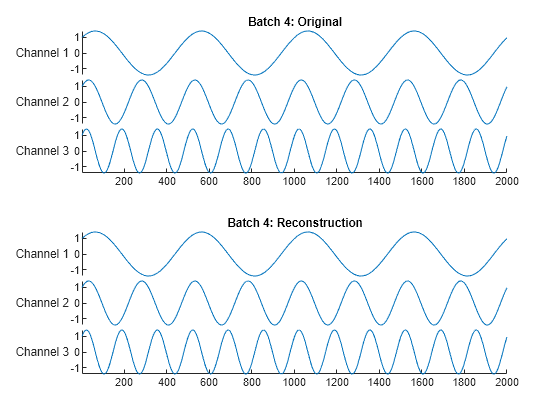
Confirm perfect reconstruction of the data.
Since R2025a
Initialize inverse short-time Fourier transform (ISTFT) layer weights to window, update deep learning neural network and reset learnable parameters.
Define an array of seven layers: a sequence input layer, an STFT layer, a 2-D convolutional layer, a batch normalization layer, a rectified linear unit (ReLU) layer, a fully connected layer, and an ISTFT layer. There is one feature in the sequence input. Set the minimum signal length in the sequence input layer to 512 samples. Use a 256-sample Hamming window, and an overlap length of 128 samples for the STFT and ISTFT layers.
win = hamming(256); ol = 128; targetLayerName = "istft"; layers = [ sequenceInputLayer(1,MinLength=512) stftLayer(Window=win,OverlapLength=ol,Name="stft") convolution2dLayer(4,16,Padding="same") batchNormalizationLayer reluLayer fullyConnectedLayer(258) istftLayer(Window=win,OverlapLength=ol,Name="istft")];
Create a deep learning neural network from the layer array. By default, the dlnetwork function initializes the network at creation. For reproducibility, use the default random number generator.
rng("default") net = dlnetwork(layers);
Display the table of learnable parameters. The network weights and bias are nonempty dlarray objects.
tInit1=8×3 table
Layer Parameter Value
___________ _________ ____________________
"stft"         "Weights"    {256×1      dlarray}
"conv"         "Weights"    {  4×4×1×16 dlarray}
"conv"         "Bias"       {  1×1×16   dlarray}
"batchnorm"    "Offset"     {  1×16     dlarray}
"batchnorm"    "Scale"      {  1×16     dlarray}
"fc"           "Weights"    {258×2064   dlarray}
"fc"           "Bias"       {258×1      dlarray}
"istft"        "Weights"    {256×1      dlarray}
Compare the initialized weights of the ISTFT layer from the list of learnable parameters with the Window property of the ISTFT layer. The istftLayer weights are single precision and initialized to the specified window.
isequal(tInit1.Value{8},single(net.Layers(7).Window))
Set the learnable parameters to empty arrays.
net = dlupdate(@(x)[],net); net.Learnables
ans=8×3 table
Layer Parameter Value
___________ _________ ____________
"stft"         "Weights"    {0×0 double}
"conv"         "Weights"    {0×0 double}
"conv"         "Bias"       {0×0 double}
"batchnorm"    "Offset"     {0×0 double}
"batchnorm"    "Scale"      {0×0 double}
"fc"           "Weights"    {0×0 double}
"fc"           "Bias"       {0×0 double}
"istft"        "Weights"    {0×0 double}
Reinitialize the network. Display the network and the learnable parameters. The network weights and bias are nonempty dlarray objects.
net = initialize(net); tInit2 = net.Learnables
tInit2=8×3 table
Layer Parameter Value
___________ _________ ____________________
"stft"         "Weights"    {256×1      dlarray}
"conv"         "Weights"    {  4×4×1×16 dlarray}
"conv"         "Bias"       {  1×1×16   dlarray}
"batchnorm"    "Offset"     {  1×16     dlarray}
"batchnorm"    "Scale"      {  1×16     dlarray}
"fc"           "Weights"    {258×2064   dlarray}
"fc"           "Bias"       {258×1      dlarray}
"istft"        "Weights"    {256×1      dlarray}
Compare the weights from the ISTFT and 2-D convolutional layers along the two initialization calls. The ISTFT layer sets the weights using the specified window, while the convolutional layer weights consists of a new set of random values.
tiledlayout flow nexttile plot(tInit1.Value{8}) hold on plot(tInit2.Value{8},"--") hold off title("ISTFT Weights (Window)") legend(["First" "Second"] + " Initialization") nexttile plot([tInit1.Value{2}(:) tInit2.Value{2}(:)]) title("2-D Convolutional Weights") legend(["First" "Second"] + " Initialization")

More About
To compute the inverse short-time Fourier transform, take the IFFT of each DFT vector of the STFT and overlap-add the inverted signals.
Recall that the STFT of a signal is computed by sliding an_analysis window_ g(n) of length M over the signal and calculating the discrete Fourier transform (DFT) of each segment of windowed data. The window hops over the original signal at intervals of R samples, equivalent to L = M –R samples of overlap between adjoining segments. The ISTFT is calculated as follows.
where Xm is the DFT of the windowed data centered about time mR and xm(n)=x(n) g(n−mR). The inverse STFT is a perfect reconstruction of the original signal as long as ∑m=−∞∞ga+1(n−mR)=c, ∀n∈ℤ, where c is a nonzero constant and a equals 0 or 1. For more information, see Constant Overlap-Add (COLA) Constraint. This figure depicts the steps in reconstructing the original signal.
To ensure successful reconstruction of nonmodified spectra, the analysis window must satisfy the COLA constraint. In general, if the analysis window satisfies the condition ∑m=−∞∞ga+1(n−mR)=c, ∀n∈ℤ, where c is a nonzero constant and a equals 0 or 1, the window is considered to be COLA-compliant. Additionally, COLA compliance can be described as either weak or strong.
- Weak COLA compliance implies that the Fourier transform of the analysis window has zeros at frame-rate harmonics such that
Alias cancellation is disturbed by spectral modifications. Weak COLA relies on alias cancellation in the frequency domain. Therefore, perfect reconstruction is possible using weakly COLA-compliant windows as long as the signal has not undergone any spectral modifications. - For strong COLA compliance, the Fourier transform of the window must be bandlimited consistently with downsampling by the frame rate such that
This equation shows that no aliasing is allowed by the strong COLA constraint. Additionally, for strong COLA compliance, the value of the constant c must equal 1. In general, if the short-time spectrum is modified in any way, a stronger COLA compliant window is preferred.
You can use the iscola function to check for weak COLA compliance. The number of summations used to check COLA compliance is dictated by the window length and hop size. In general, it is common to use a=1 in ∑m=−∞∞ga+1(n−mR)=c, ∀n∈ℤ, for weighted overlap-add (WOLA), and a=0 for overlap-add (OLA). By default, istft uses the WOLA method, by applying a synthesis window before performing the overlap-add method.
In general, the synthesis window is the same as the analysis window. You can construct useful WOLA windows by taking the square root of a strong OLA window. You can use this method for all nonnegative OLA windows. For example, the root-Hann window is a good example of a WOLA window.
In general, computing the STFT of an input signal and inverting it does not result in perfect reconstruction. If you want the output of ISTFT to match the original input signal as closely as possible, the signal and the window must satisfy the following conditions:
- Input size — If you invert the output of
stftusingistftand want the result to be the same length as the input signalx, the value of
must be an integer. In the equation,Nx is the length of the signal, M is the length of the window, and_L_ is the overlap length. - COLA compliance — Use COLA-compliant windows, assuming that you have not modified the short-time Fourier transform of the signal.
- Padding — If the length of the input signal is such that the value of_k_ is not an integer, zero-pad the signal before computing the short-time Fourier transform. Remove the extra zeros after inverting the signal.
You can use the stftmag2sig function to obtain an estimate of a signal reconstructed from the magnitude of its STFT.
The input to istftLayer must be a real-valueddlarray object in "CBT" or "SCBT" format. The output is a real-valued "CBT" array.
If the input is in "SCBT" format, the "S" dimension corresponds to frequency.
If the input is in "CBT" format, istftLayer assumes the frequency and channel dimensions have been flattened into the channel dimension.
Algorithms
The size of the ISTFT depends on the dimensions and data format of the input STFT, the length of the windowing function, the number of overlapped samples and the number of DFT points.
Define the hop size as hopSize = length(`Window`)-`OverlapLength`. The number of samples in the ISTFT islength(`Window`)+(nseg-1)*hopSize, wherenseg is the size of the input in the time ("T") dimension.
- If the input to
istftLayeris a"SCBT"formatteddlarray, the number of channels isszC/2, whereszCis the size of the input in the channel ("C") dimension. - If the input to
istftLayeris a"CBT"formatteddlarray, the number of channels isszC/(2*nfreq), wherenfreq = floor(`FFTLength`/2)+1.
Extended Capabilities
Usage notes and limitations:
- You can generate generic C/C++ code that does not depend on third-party libraries and deploy the generated code to hardware platforms.
Usage notes and limitations:
- You can generate CUDA code that is independent of deep learning libraries and deploy the generated code to platforms that use NVIDIA® GPU processors.
Version History
Introduced in R2024a
Starting in R2025a, you can use initialize (Deep Learning Toolbox) to initialize learnable parameters for deep learning neural networks that includeistftLayer objects.
Starting in R2025a, the default value of the Weights property is[]. Prior to R2025a, istftLayer set the default value to the synthesis window used to compute the transform.
The istftLayer object supports:
- C/C++ code generation. You must have MATLAB® Coder™ to generate C/C++ code.
- Code generation for NVIDIA GPUs. You must have GPU Coder™ to generate GPU code.
See Also
Apps
- Deep Network Designer (Deep Learning Toolbox)