pspectrum - Analyze signals in the frequency and time-frequency domains - MATLAB (original) (raw)
Analyze signals in the frequency and time-frequency domains
Syntax
Description
[p](#d126e191576) = pspectrum([x](#d126e190959)) returns the power spectrum of x.
- If
xis a vector or a timetable with a vector of data, then it is treated as a single channel. - If
xis a matrix, a timetable with a matrix variable, or a timetable with multiple vector variables, then the spectrum is computed independently for each channel and stored in a separate column ofp.
[p](#d126e191576) = pspectrum([x](#d126e190959),[fs](#d126e191038)) returns the power spectrum of a vector or matrix signal sampled at a ratefs.
[p](#d126e191576) = pspectrum([x](#d126e190959),[t](#d126e191059)) returns the power spectrum of a vector or matrix signal sampled at the time instants specified in t.
[p](#d126e191576) = pspectrum(___,[type](#d126e191111)) specifies the kind of spectral analysis performed by the function. Specifytype as 'power','spectrogram', or 'persistence'. This syntax can include any combination of input arguments from previous syntaxes.
[p](#d126e191576) = pspectrum(___,[Name,Value](#namevaluepairarguments)) specifies additional options using name-value pair arguments. Options include the frequency resolution bandwidth and the percent overlap between adjoining segments.
[[p](#d126e191576),[f](#d126e191684)] = pspectrum(___) returns the frequencies corresponding to the spectral estimates contained inp.
[[p](#d126e191576),[f](#d126e191684),[t](pspectrum.html#mw%5Fe554f022-56f0-44a7-8976-c59bab64715c)] = pspectrum(___,'spectrogram') also returns a vector of time instants corresponding to the centers of the windowed segments used to compute short-time power spectrum estimates.
[[p](#d126e191576),[f](#d126e191684),[pwr](#d126e191772)] = pspectrum(___,'persistence') also returns a vector of power values corresponding to the estimates contained in a persistence spectrum.
pspectrum(___) with no output arguments plots the spectral estimate in the current figure window. For the plot, the function converts p to dB using 10 log10(p).
Examples
Generate 128 samples of a two-channel complex sinusoid.
- The first channel has unit amplitude and a normalized sinusoid frequency of π/4 rad/sample
- The second channel has an amplitude of 1/2 and a normalized frequency of π/2 rad/sample.
Compute and plot the power spectrum of each channel. Zoom in on the frequency range from 0.15π rad/sample to 0.6π rad/sample. pspectrum scales the spectrum so that, if the frequency content of a signal falls exactly within a bin, its amplitude in that bin is the true average power of the signal. For a complex exponential, the average power is the square of the amplitude. Verify by computing the discrete Fourier transform of the signal. For more details, see Measure Power of Deterministic Periodic Signals.
N = 128; x = [1 1/sqrt(2)].exp(1jpi./[4;2]*(0:N-1)).';
[p,f] = pspectrum(x);
plot(f/pi,p) hold on stem(0:2/N:2-1/N,abs(fft(x)/N).^2) hold off axis([0.15 0.6 0 1.1]) legend("Channel "+[1;2]+", "+["pspectrum" "fft"]) grid

Generate a sinusoidal signal sampled at 1 kHz for 296 milliseconds and embedded in white Gaussian noise. Specify a sinusoid frequency of 200 Hz and a noise variance of 0.1². Store the signal and its time information in a MATLAB® timetable.
Fs = 1000; t = (0:1/Fs:0.296)'; x = cos(2pit200)+0.1randn(size(t)); xTable = timetable(seconds(t),x);
Compute the power spectrum of the signal. Express the spectrum in decibels and plot it.
[pxx,f] = pspectrum(xTable);
plot(f,pow2db(pxx)) grid on xlabel('Frequency (Hz)') ylabel('Power Spectrum (dB)') title('Default Frequency Resolution')

Recompute the power spectrum of the sinusoid, but now use a coarser frequency resolution of 25 Hz. Plot the spectrum using the pspectrum function with no output arguments.
pspectrum(xTable,'FrequencyResolution',25)

Generate a signal sampled at 3 kHz for 1 second. The signal is a convex quadratic chirp whose frequency increases from 300 Hz to 1300 Hz during the measurement. The chirp is embedded in white Gaussian noise.
fs = 3000; t = 0:1/fs:1-1/fs;
x1 = chirp(t,300,t(end),1300,'quadratic',0,'convex') + ... randn(size(t))/100;
Compute and plot the two-sided power spectrum of the signal using a rectangular window. For real signals, pspectrum plots a one-sided spectrum by default. To plot a two-sided spectrum, set TwoSided to true.
pspectrum(x1,fs,'Leakage',1,'TwoSided',true)

Generate a complex-valued signal with the same duration and sample rate. The signal is a chirp with sinusoidally varying frequency content and embedded in white noise. Compute the spectrogram of the signal and display it as a waterfall plot. For complex-valued signals, the spectrogram is two-sided by default.
x2 = exp(2jpi100cos(2pi2t)) + randn(size(t))/100;
[p,f,t] = pspectrum(x2,fs,'spectrogram');
waterfall(f,t,p') xlabel('Frequency (Hz)') ylabel('Time (seconds)') wtf = gca; wtf.XDir = 'reverse'; view([30 45])

Generate a two-channel signal sampled at 100 Hz for 2 seconds.
- The first channel consists of a 20 Hz tone and a 21 Hz tone. Both tones have unit amplitude.
- The second channel also has two tones. One tone has unit amplitude and a frequency of 20 Hz. The other tone has an amplitude of 1/100 and a frequency of 30 Hz.
fs = 100; t = (0:1/fs:2-1/fs)';
x = sin(2pi[20 20].t) + [1 1/100].sin(2pi[21 30].*t);
Embed the signal in white noise. Specify a signal-to-noise ratio of 40 dB. Plot the signals.
x = x + randn(size(x)).*std(x)/db2mag(40);
plot(t,x)

Compute the spectra of the two channels and display them.

The default value for the spectral leakage, 0.5, corresponds to a resolution bandwidth of about 1.29 Hz. The two tones in the first channel are not resolved. The 30 Hz tone in the second channel is visible, despite being much weaker than the other one.
Increase the leakage to 0.85, equivalent to a resolution of about 0.74 Hz. The weak tone in the second channel is clearly visible.
pspectrum(x,t,'Leakage',0.85)

Increase the leakage to the maximum value. The resolution bandwidth is approximately 0.5 Hz. The two tones in the first channel are resolved. The weak tone in the second channel is masked by the large window sidelobes.
pspectrum(x,t,'Leakage',1)

Generate a signal that consists of a voltage-controlled oscillator and three Gaussian atoms. The signal is sampled at fs=2 kHz for 2 seconds.
fs = 2000; tx = 0:1/fs:2; gaussFun = @(A,x,mu,f) exp(-(x-mu).^2/(20.03^2)).sin(2pif.*x)*A'; s = gaussFun([1 1 1],tx',[0.1 0.65 1],[2 6 2]*100)*1.5; x = vco(chirp(tx+.1,0,tx(end),3).exp(-2(tx-1).^2),[0.1 0.4]*fs,fs); x = s+x';
Short-Time Fourier Transforms
Use the pspectrum function to compute the STFT.
- Divide the Nx-sample signal into segments of length M=80 samples, corresponding to a time resolution of 80/2000=40 milliseconds.
- Specify L=16 samples or 20% of overlap between adjoining segments.
- Window each segment with a Kaiser window and specify a leakage ℓ=0.7.
M = 80; L = 16; lk = 0.7;
[S,F,T] = pspectrum(x,fs,"spectrogram", ... TimeResolution=M/fs,OverlapPercent=L/M*100, ... Leakage=lk);
Compare to the result obtained with the spectrogram function.
- Specify the window length and overlap directly in samples.
pspectrumalways uses a Kaiser window as g(n). The leakage ℓ and the shape factor β of the window are related by β=40×(1-ℓ).pspectrumalways uses NDFT=1024 points when computing the discrete Fourier transform. You can specify this number if you want to compute the transform over a two-sided or centered frequency range. However, for one-sided transforms, which are the default for real signals,spectrogramuses 1024/2+1=513 points. Alternatively, you can specify the vector of frequencies at which you want to compute the transform, as in this example.- If a signal cannot be divided exactly into k=⌊Nx-LM-L⌋ segments,
spectrogramtruncates the signal whereaspspectrumpads the signal with zeros to create an extra segment. To make the outputs equivalent, remove the final segment and the final element of the time vector. spectrogramreturns the STFT, whose magnitude squared is the spectrogram.pspectrumreturns the segment-by-segment power spectrum, which is already squared but is divided by a factor of ∑ng(n) before squaring.- For one-sided transforms,
pspectrumadds an extra factor of 2 to the spectrogram.
g = kaiser(M,40*(1-lk));
k = (length(x)-L)/(M-L); if k~=floor(k) S = S(:,1:floor(k)); T = T(1:floor(k)); end
[s,f,t] = spectrogram(x/sum(g)*sqrt(2),g,L,F,fs);
Use the waterplot function to display the spectrograms computed by the two functions.
subplot(2,1,1) waterplot(sqrt(S),F,T) title("pspectrum")
subplot(2,1,2) waterplot(s,f,t) title("spectrogram")
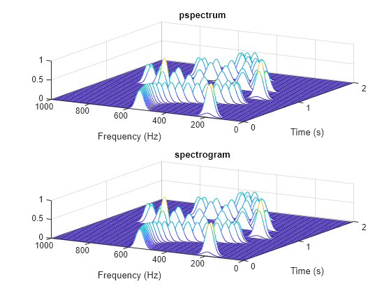
maxd = max(max(abs(abs(s).^2-S)))
Power Spectra and Convenience Plots
The spectrogram function has a fourth argument that corresponds to the segment-by-segment power spectrum or power spectral density. Similar to the output of pspectrum, the ps argument is already squared and includes the normalization factor ∑ng(n). For one-sided spectrograms of real signals, you still have to include the extra factor of 2. Set the scaling argument of the function to "power".
[,,~,ps] = spectrogram(x*sqrt(2),g,L,F,fs,"power");
max(abs(S(:)-ps(:)))
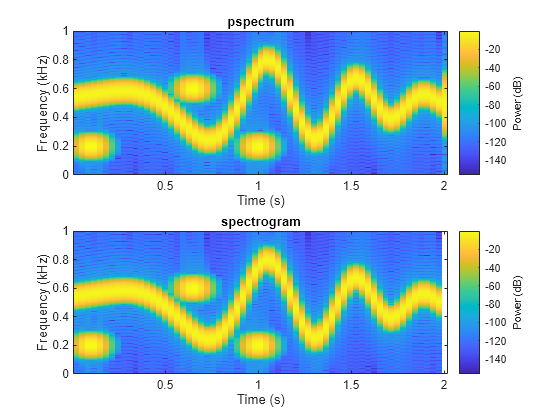
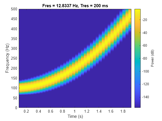
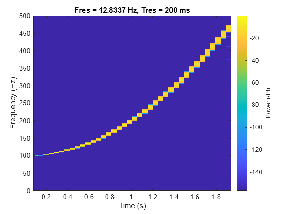
When called with no output arguments, both pspectrum and spectrogram plot the spectrogram of the signal in decibels. Include the factor of 2 for one-sided spectrograms. Set the colormaps to be the same for both plots. Set the _x_-limits to the same values to make visible the extra segment at the end of the pspectrum plot. In the spectrogram plot, display the frequency on the _y_-axis.
subplot(2,1,1) pspectrum(x,fs,"spectrogram", ... TimeResolution=M/fs,OverlapPercent=L/M*100, ... Leakage=lk) title("pspectrum") cc = clim; xl = xlim;
subplot(2,1,2) spectrogram(x*sqrt(2),g,L,F,fs,"power","yaxis") title("spectrogram") clim(cc) xlim(xl)
function waterplot(s,f,t) % Waterfall plot of spectrogram waterfall(f,t,abs(s)'.^2) set(gca,XDir="reverse",View=[30 50]) xlabel("Frequency (Hz)") ylabel("Time (s)") end
Visualize an interference narrowband signal embedded within a broadband signal.
Generate a chirp sampled at 1 kHz for 500 seconds. The frequency of the chirp increases from 180 Hz to 220 Hz during the measurement.
fs = 1000; t = (0:1/fs:500)';
x = chirp(t,180,t(end),220) + 0.15*randn(size(t));
The signal also contains a 210 Hz sinusoid. The sinusoid has an amplitude of 0.05 and is present only for 1/6 of the total signal duration.
idx = floor(length(x)/6); x(1:idx) = x(1:idx) + 0.05cos(2pi*t(1:idx)*210);
Compute the spectrogram of the signal. Restrict the frequency range from 100 Hz to 290 Hz. Specify a time resolution of 1 second. Both signal components are visible.
pspectrum(x,fs,'spectrogram', ... 'FrequencyLimits',[100 290],'TimeResolution',1)

Compute the power spectrum of the signal. The weak sinusoid is obscured by the chirp.
pspectrum(x,fs,'FrequencyLimits',[100 290])

Compute the persistence spectrum of the signal. Now both signal components are clearly visible.
pspectrum(x,fs,'persistence', ... 'FrequencyLimits',[100 290],'TimeResolution',1)

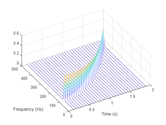
Generate a quadratic chirp sampled at 1 kHz for 2 seconds. The chirp has an initial frequency of 100 Hz that increases to 200 Hz at t = 1 second. Compute the spectrogram using the default settings of the pspectrum function. Use the waterfall function to plot the spectrogram.
fs = 1e3; t = 0:1/fs:2; y = chirp(t,100,1,200,"quadratic");
[sp,fp,tp] = pspectrum(y,fs,"spectrogram");
waterfall(fp,tp,sp') set(gca,XDir="reverse",View=[60 60]) ylabel("Time (s)") xlabel("Frequency (Hz)")
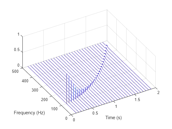
Compute and display the reassigned spectrogram.
[sr,fr,tr] = pspectrum(y,fs,"spectrogram",Reassign=true);
waterfall(fr,tr,sr') set(gca,XDir="reverse",View=[60 60]) ylabel("Time (s)") xlabel("Frequency (Hz)")
Recompute the spectrogram using a time resolution of 0.2 second. Visualize the result using the pspectrum function with no output arguments.
pspectrum(y,fs,"spectrogram",TimeResolution=0.2)
Compute the reassigned spectrogram using the same time resolution.
pspectrum(y,fs,"spectrogram",TimeResolution=0.2,Reassign=true)
Create a signal, sampled at 4 kHz, that resembles pressing all the keys of a digital telephone. Save the signal as a MATLAB® timetable.
fs = 4e3; t = 0:1/fs:0.5-1/fs;
ver = [697 770 852 941]; hor = [1209 1336 1477];
tones = [];
for k = 1:length(ver) for l = 1:length(hor) tone = sum(sin(2pi[ver(k);hor(l)].*t))'; tones = [tones;tone;zeros(size(tone))]; end end
% To hear, type soundsc(tones,fs)
S = timetable(seconds(0:length(tones)-1)'/fs,tones);
Compute the spectrogram of the signal. Specify a time resolution of 0.5 second and zero overlap between adjoining segments. Specify the leakage as 0.85, which is approximately equivalent to windowing the data with a Hann window.
pspectrum(S,'spectrogram', ... 'TimeResolution',0.5,'OverlapPercent',0,'Leakage',0.85)
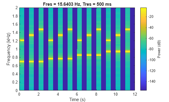
The spectrogram shows that each key is pressed for half a second, with half-second silent pauses between keys. The first tone has a frequency content concentrated around 697 Hz and 1209 Hz, corresponding to the digit '1' in the DTMF standard.
Input Arguments
Input signal, specified as a vector, a matrix, or a MATLAB® timetable.
- If
xis a timetable, then it must contain increasing finite row times. - If
xis a timetable representing a multichannel signal, then it must have either a single variable containing a matrix or multiple variables consisting of vectors.
If x is nonuniformly sampled, thenpspectrum interpolates the signal to a uniform grid to compute spectral estimates. The function uses linear interpolation and assumes a sample time equal to the median of the differences between adjacent time points. For a nonuniformly sampled signal to be supported, the median time interval and the mean time interval must obey
Example: cos(pi./[4;2]*(0:159))'+randn(160,2) is a two-channel signal consisting of sinusoids embedded in white noise.
Example: timetable(seconds(0:4)',rand(5,2)) specifies a two-channel random variable sampled at 1 Hz for 4 seconds.
Example: timetable(seconds(0:4)',rand(5,1),rand(5,1)) specifies a two-channel random variable sampled at 1 Hz for 4 seconds.
Data Types: single | double
Complex Number Support: Yes
Sample rate, specified as a positive numeric scalar.
Time values, specified as a vector, a datetime or duration array, or aduration scalar representing the time interval between samples.
Example: seconds(0:1/100:1) is a`duration` array representing 1 second of sampling at 100 Hz.
Example: seconds(1) is a`duration` scalar representing a 1-second time difference between consecutive signal samples.
Type of spectrum to compute, specified as 'power','spectrogram', or 'persistence':
'power'— Compute the power spectrum of the input. Use this option to analyze the frequency content of a stationary signal. For more information, Spectrum Computation.'spectrogram'— Compute the spectrogram of the input. Use this option to analyze how the frequency content of a signal changes over time. For more information, see Spectrogram Computation.'persistence'— Compute the persistence power spectrum of the input. Use this option to visualize the fraction of time that a particular frequency component is present in a signal. For more information, see Persistence Spectrum Computation.
Note
The 'spectrogram' and'persistence' options do not support multichannel input.
Name-Value Arguments
Specify optional pairs of arguments asName1=Value1,...,NameN=ValueN, where Name is the argument name and Value is the corresponding value. Name-value arguments must appear after other arguments, but the order of the pairs does not matter.
Before R2021a, use commas to separate each name and value, and enclose Name in quotes.
Example: 'Leakage',1,'Reassign',true,'MinThreshold',-35 windows the data using a rectangular window, computes a reassigned spectrum estimate, and sets all values smaller than –35 dB to zero.
Frequency band limits, specified as the comma-separated pair consisting of 'FrequencyLimits' and a two-element numeric vector:
- If the input contains time information, then the frequency band is expressed in Hz.
- If the input does not contain time information, then the frequency band is expressed in normalized units of rad/sample.
By default, pspectrum computes the spectrum over the whole Nyquist range:
- If the specified frequency band contains a region that falls outside the Nyquist range, then
pspectrumtruncates the frequency band. - If the specified frequency band lies completely outside of the Nyquist range, then
pspectrumthrows an error.
See Spectrum Computation for more information about the Nyquist range.
If x is nonuniformly sampled, thenpspectrum linearly interpolates the signal to a uniform grid and defines an effective sample rate equal to the inverse of the median of the differences between adjacent time points. Express'FrequencyLimits' in terms of the effective sample rate.
Example: [0.2*pi 0.7*pi] computes the spectrum between 0.2_π_ rad/sample and 0.7_π_ rad/sample of a signal with no time information.
Frequency resolution bandwidth, specified as the comma-separated pair consisting of 'FrequencyResolution' and a real numeric scalar, expressed in Hz if the input contains time information, or in normalized units of rad/sample if not. This argument cannot be specified simultaneously with 'TimeResolution'. The default value of this argument depends on the size of the input data. See Spectrogram Computation for details.
Example: pi/100 computes the spectrum of a signal with no time information using a frequency resolution of_π_/100 rad/sample.
Spectral leakage, specified as the comma-separated pair consisting of'Leakage' and a real numeric scalar between 0 and 1. 'Leakage' controls the Kaiser window sidelobe attenuation relative to the mainlobe width, balancing between improving resolution and decreasing leakage:
- A large leakage value resolves closely spaced tones, but masks nearby weak tones.
- A small leakage value finds small tones in the vicinity of larger tones, but smears close frequencies together.
Example: 'Leakage',0 reduces leakage to a minimum at the expense of spectral resolution.
Example: 'Leakage',0.85 approximates windowing the data with a Hann window.
Example: 'Leakage',1 is equivalent to windowing the data with a rectangular window, maximizing leakage but improving spectral resolution.
Lower bound for nonzero values, specified as the comma-separated pair consisting of 'MinThreshold' and a real scalar.pspectrum implements'MinThreshold' differently based on the value of the type argument:
'power'or'spectrogram'—pspectrumsets those elements ofp such that 10 log10(p) ≤'MinThreshold'to zero. Specify'MinThreshold'in decibels.'persistence'—pspectrumsets those elements ofpsmaller than'MinThreshold'to zero. Specify'MinThreshold'between 0 and 100%.
Number of power bins for persistence spectrum, specified as the comma-separated pair consisting of 'NumPowerBins' and an integer between 20 and 1024.
Overlap between adjoining segments for spectrogram or persistence spectrum, specified as the comma-separated pair consisting of'OverlapPercent' and a real scalar in the interval [0, 100). The default value of this argument depends on the spectral window. See Spectrogram Computation for details.
Reassignment option, specified as the comma-separated pair consisting of 'Reassign' and a logical value. If this option is set to true, then pspectrum sharpens the localization of spectral estimates by performing time and frequency reassignment. The reassignment technique produces periodograms and spectrograms that are easier to read and interpret. This technique reassigns each spectral estimate to the center of energy of its bin instead of the bin's geometric center. The technique provides exact localization for chirps and impulses.
Time resolution of spectrogram or persistence spectrum, specified as the comma-separated pair consisting of'TimeResolution' and a real scalar, expressed in seconds if the input contains time information, or as an integer number of samples if not. This argument controls the duration of the segments used to compute the short-time power spectra that form spectrogram or persistence spectrum estimates. 'TimeResolution' cannot be specified simultaneously with'FrequencyResolution'. The default value of this argument depends on the size of the input data and, if it was specified, the frequency resolution. See Spectrogram Computation for details.
Two-sided spectral estimate, specified as the comma-separated pair consisting of 'TwoSided' and a logical value.
- If this option is
true, the function computes centered, two-sided spectrum estimates over [–π,_π_]. If the input has time information, the estimates are computed over [–_f_s/2,_f_s/2], where_f_s is the effective sample rate. - If this option is
false, the function computes one-sided spectrum estimates over the Nyquist range [0, _π_]. If the input has time information, the estimates are computed over [0,_f_s/2], where_f_s is the effective sample rate. To conserve the total power, the function multiplies the power by 2 at all frequencies except 0 and the Nyquist frequency. This option is valid only for real signals.
If not specified, 'TwoSided' defaults to false for real input signals and totrue for complex input signals.
Output Arguments
Spectrum, returned as a vector or a matrix. The type and size of the spectrum depends on the value of the type argument:
'power'—pcontains the power spectrum estimate of each channel ofx. In this case,pis of size_N_f × _N_ch, where _N_f is the length of f and_N_ch is the number of channels ofx.pspectrumscales the spectrum so that, if the frequency content of a signal falls exactly within a bin, its amplitude in that bin is the true average power of the signal. For example, the average power of a sinusoid is one-half the square of the sinusoid amplitude. For more details, seeMeasure Power of Deterministic Periodic Signals.'spectrogram'—pcontains an estimate of the short-term, time-localized power spectrum ofx. In this case,pis of size_N_f × _N_t, where _N_f is the length offand_N_t is the length of t.'persistence'—pcontains, expressed as percentages, the probabilities that the signal has components of a given power level at a given time and frequency location. In this case,pis of size_N_pwr × _N_f, where _N_pwr is the length of pwr and_N_f is the length off.
Spectrum frequencies, returned as a vector. If the input signal contains time information, then f contains frequencies expressed in Hz. If the input signal does not contain time information, then the frequencies are in normalized units of rad/sample.
Time values of spectrogram, returned as a vector of time values in seconds or a duration array. If the input does not have time information, then t contains sample numbers. t contains the time values corresponding to the centers of the data segments used to compute short-time power spectrum estimates.
- If the input to
pspectrumis a timetable, then t has the same format as the time values of the input timetable. - If the input to
pspectrumis a numeric vector sampled at a set of time instants specified by a numeric,duration, ordatetime array, then t has the same type and format as the input time values. - If the input to
pspectrumis a numeric vector with a specified time difference between consecutive samples, then t is a duration array.
Power values of persistence spectrum, returned as a vector.
More About
To compute signal spectra, pspectrum finds a compromise between the spectral resolution achievable with the entire length of the signal and the performance limitations that result from computing large FFTs:
- If possible, the function computes a single modified periodogram of the whole signal using a Kaiser window.
- If it is not possible to compute a single modified periodogram in a reasonable amount of time, the function computes a Welch periodogram: It divides the signal into overlapping segments, windows each segment using a Kaiser window, and averages the periodograms of the segments.
Spectral Windowing
Any real-world signal is measurable only for a finite length of time. This fact introduces nonnegligible effects into Fourier analysis, which assumes that signals are either periodic or infinitely long. Spectral windowing, which assigns different weights to different signal samples, deals systematically with finite-size effects.
The simplest way to window a signal is to assume that it is identically zero outside of the measurement interval and that all samples are equally significant. This "rectangular window" has discontinuous jumps at both ends that result in spectral ringing. All other spectral windows taper at both ends to lessen this effect by assigning smaller weights to samples close to the signal edges.
The windowing process always involves a compromise between conflicting aims: improving resolution and decreasing leakage:
- Resolution is the ability to know precisely how the signal energy is distributed in the frequency space. A spectrum analyzer with ideal resolution can distinguish two different tones (pure sinusoids) present in the signal, no matter how close in frequency. Quantitatively, this ability relates to the mainlobe width of the transform of the window.
- Leakage is the fact that, in a finite signal, every frequency component projects energy content throughout the complete frequency span. The amount of leakage in a spectrum can be measured by the ability to detect a weak tone from noise in the presence of a neighboring strong tone. Quantitatively, this ability relates to the sidelobe level of the frequency transform of the window.
- The spectrum is normalized so that a pure tone within that bandwidth, if perfectly centered, has the correct amplitude.
The better the resolution, the higher the leakage, and vice versa. At one end of the range, a rectangular window has the narrowest possible mainlobe and the highest sidelobes. This window can resolve closely spaced tones if they have similar energy content, but it fails to find the weaker one if they do not. At the other end, a window with high sidelobe suppression has a wide mainlobe in which close frequencies are smeared together.
pspectrum uses Kaiser windows to carry out windowing. For Kaiser windows, the fraction of the signal energy captured by the mainlobe depends most importantly on an adjustable shape factor,β. pspectrum uses shape factors ranging from β = 0, which corresponds to a rectangular window, to β = 40, where a wide mainlobe captures essentially all the spectral energy representable in double precision. An intermediate value of β ≈ 6 approximates a Hann window quite closely. To control_β_, use the 'Leakage' name-value pair. If you set 'Leakage' to ℓ, then_ℓ_ and β are related by β = 40(1 – ℓ). See kaiser for more details.
 |
 |
|---|---|
| 51-point Hann window and 51-point Kaiser window with β = 5.7 in the time domain | 51-point Hann window and 51-point Kaiser window with β = 5.7 in the frequency domain |
Parameter and Algorithm Selection
To compute signal spectra, pspectrum initially determines the_resolution bandwidth_, which measures how close two tones can be and still be resolved. The resolution bandwidth has a theoretical value of
- _t_max –_t_min, the record length, is the time-domain duration of the selected signal region.
- ENBW is the equivalent noise bandwidth of the spectral window. See enbw for more details.
Use the'Leakage'name-value pair to control the ENBW. The minimum value of the argument corresponds to a Kaiser window with β = 40. The maximum value corresponds to a Kaiser window with β = 0.
In practice, however, pspectrum might lower the resolution. Lowering the resolution makes it possible to compute the spectrum in a reasonable amount of time and to display it with a finite number of pixels. For these practical reasons, the lowest resolution bandwidth pspectrum can use is
where _f_span is the width of the frequency band specified using'FrequencyLimits'. If'FrequencyLimits' is not specified, thenpspectrum uses the sample rate as _f_span. RBWperformance cannot be adjusted.
To compute the spectrum of a signal, the function chooses the larger of the two values, called the target resolution bandwidth:
- If the resolution bandwidth is RBWtheory, then
pspectrumcomputes a single_modified periodogram_ for the whole signal. The function uses a Kaiser window with shape factor controlled by the'Leakage'name-value pair. See periodogram for more details. - If the resolution bandwidth is RBWperformance, then
pspectrumcomputes a_Welch periodogram_ for the signal. The function:- Divides the signals into overlapping segments.
- Windows each segment separately using a Kaiser window with the specified shape factor.
- Averages the periodograms of all the segments.
Welch’s procedure is designed to reduce the variance of the spectrum estimate by averaging different “realizations” of the signals, given by the overlapping sections, and using the window to remove redundant data. See pwelch for more details.
- The length of each segment (or, equivalently, of the window) is computed using
where _f_Nyquist is the Nyquist frequency. (If there is no aliasing, the Nyquist frequency is one-half the effective sample rate, defined as the inverse of the median of the differences between adjacent time points. The Nyquist range is [0,_f_Nyquist] for real signals and [–_f_Nyquist,_f_Nyquist] for complex signals.) - The stride length is found by adjusting an initial estimate,
so that the first window starts exactly on the first sample of the first segment and the last window ends exactly on the last sample of the last segment.
To compute the time-dependent spectrum of a nonstationary signal,pspectrum divides the signal into overlapping segments, windows each segment with a Kaiser window, computes the short-time Fourier transform, and then concatenates the transforms to form a matrix. For more information, see Spectrogram Computation with Signal Processing Toolbox.
A nonstationary signal is a signal whose frequency content changes with time. The_spectrogram_ of a nonstationary signal is an estimate of the time evolution of its frequency content. To construct the spectrogram of a nonstationary signal, pspectrum follows these steps:
- Divide the signal into equal-length segments. The segments must be short enough that the frequency content of the signal does not change appreciably within a segment. The segments may or may not overlap.
- Window each segment and compute its spectrum to get the_short-time Fourier transform_.
- Use the segment spectra to construct the spectrogram:
- If called with output arguments, concatenate the spectra to form a matrix.
- If called with no output arguments, display the power of each spectrum in decibels segment by segment. Depict the magnitudes side-by-side as an image with magnitude-dependent colormap.
The function can compute the spectrogram only for single-channel signals.
Divide Signal into Segments
To construct a spectrogram, first divide the signal into possibly overlapping segments. With the pspectrum function, you can control the length of the segments and the amount of overlap between adjoining segments using the 'TimeResolution' and 'OverlapPercent' name-value pair arguments. If you do not specify the length and overlap, the function chooses a length based on the entire length of the signal and an overlap percentage given by
where ENBW is the equivalent noise bandwidth of the spectral window. See enbw and Spectrum Computation for more information.
Specified Time Resolution
- If the signal does not have time information, specify the time resolution (segment length) in samples. The time resolution must be an integer greater than or equal to 1 and smaller than or equal to the signal length.
If the signal has time information, specify the time resolution in seconds. The function converts the result into a number of samples and rounds it to the nearest integer that is less than or equal to the number but not smaller than 1. The time resolution must be smaller than or equal to the signal duration. - Specify the overlap as a percentage of the segment length. The function converts the result into a number of samples and rounds it to the nearest integer that is less than or equal to the number.
Default Time Resolution
If you do not specify a time resolution, then pspectrum uses the length of the entire signal to choose the length of the segments. The function sets the time resolution as ⌈N/d_⌉ samples, where the ⌈⌉ symbols denote the ceiling function, N is the length of the signal, and d is a divisor that depends on_N:
| Signal Length (N) | Divisor (d) | Segment Length |
|---|---|---|
| 2 samples – 63 samples | 2 | 1 sample – 32 samples |
| 64 samples – 255 samples | 8 | 8 samples – 32 samples |
| 256 samples – 2047 samples | 8 | 32 samples – 256 samples |
| 2048 samples – 4095 samples | 16 | 128 samples – 256 samples |
| 4096 samples – 8191 samples | 32 | 128 samples – 256 samples |
| 8192 samples – 16383 samples | 64 | 128 samples – 256 samples |
| 16384 samples – N samples | 128 | 128 samples – ⌈N /128⌉ samples |
You can still specify the overlap between adjoining segments. Specifying the overlap changes the number of segments. Segments that extend beyond the signal endpoint are zero-padded.
Consider the seven-sample signal [s0 s1 s2 s3 s4 s5 s6]. Because ⌈7/2⌉ = ⌈3.5⌉ = 4, the function divides the signal into two segments of length four when there is no overlap. The number of segments changes as the overlap increases.
| Number of Overlapping Samples | Resulting Segments |
|---|---|
| 0 | s0 s1 s2 s3 s4 s5 s6 0 |
| 1 | s0 s1 s2 s3 s3 s4 s5 s6 |
| 2 | s0 s1 s2 s3 s2 s3 s4 s5 s4 s5 s6 0 |
| 3 | s0 s1 s2 s3 s1 s2 s3 s4 s2 s3 s4 s5 s3 s4 s5 s6 |
pspectrum zero-pads the signal if the last segment extends beyond the signal endpoint. The function returns t, a vector of time instants corresponding to the centers of the segments.
Window the Segments and Compute Spectra
After pspectrum divides the signal into overlapping segments, the function windows each segment with a Kaiser window. The shape factor_β_ of the window, and therefore the leakage, can be adjusted using the 'Leakage' name-value pair. The function then computes the spectrum of each segment and concatenates the spectra to form the spectrogram matrix. To compute the segment spectra, pspectrum follows the procedure described in Spectrum Computation, except that the lower limit of the resolution bandwidth is
Display Spectrum Power
If called with no output arguments, the function displays the power of the short-time Fourier transform in decibels, using a color bar with the default MATLAB colormap. The color bar comprises the full power range of the spectrogram.
The persistence spectrum is a time-frequency view that shows the percentage of the time that a given frequency is present in a signal. The persistence spectrum is a histogram in power-frequency space. The longer a particular frequency persists in a signal as the signal evolves, the higher its time percentage and thus the brighter or "hotter" its color in the display. Use the persistence spectrum to identify signals hidden in other signals.
To compute the persistence spectrum, pspectrum performs these steps:
- Compute the spectrogram using the specified leakage, time resolution, and overlap. See Spectrogram Computation for more details.
- Partition the power and frequency values into 2-D bins. (Use the
'NumPowerBins'name-value pair to specify the number of power bins.) - For each time value, compute a bivariate histogram of the logarithm of the power spectrum. For every power-frequency bin where there is signal energy at that instant, increase the corresponding matrix element by 1. Sum the histograms for all the time values.
- Plot the accumulated histogram against the power and the frequency, with the color proportional to the logarithm of the histogram counts expressed as normalized percentages. To represent zero values, use one-half of the smallest possible magnitude.
| Power Spectra |
|---|
 |
| Histograms |
 |
| Accumulated Histogram |
 |
References
[1] harris, fredric j. “On the Use of Windows for Harmonic Analysis with the Discrete Fourier Transform.” Proceedings of the IEEE®. Vol. 66, January 1978, pp. 51–83.
[2] Welch, Peter D. "The Use of Fast Fourier Transform for the Estimation of Power Spectra: A Method Based on Time Averaging Over Short, Modified Periodograms."IEEE Transactions on Audio and Electroacoustics. Vol. 15, June 1967, pp. 70–73.
Extended Capabilities
The pspectrum function supports GPU array input with these usage notes and limitations:
- Persistence spectrum is not supported.
- Reassigned spectrum or spectrogram is not supported.
For more information, see Run MATLAB Functions on a GPU (Parallel Computing Toolbox).
Version History
Introduced in R2017b
The pspectrum function supports MATLAB timetables for code generation.
You can now use the Create Plot Live Editor task to visualize the output ofpspectrum interactively. You can select different chart types and set optional parameters. The task also automatically generates code that becomes part of your live script.