Spectrogram Computation with Signal Processing Toolbox - MATLAB & Simulink (original) (raw)

Signal Processing Toolbox™ provides three functions that compute the spectrogram of a nonstationary signal. Each of the functions has different input arguments, default values, and outputs. The best choice for you depends on your particular application.

A nonstationary signal is a signal whose frequency content changes over time. The short-time Fourier transform (STFT) is used to analyze how this frequency content changes as the signal evolves. The magnitude squared of the STFT is known as the spectrogram time-frequency representation of the signal.

The spectrogram is only one of several possible time-frequency representations. For an overview of other time-frequency representations available in Signal Processing Toolbox and Wavelet Toolbox™, see Time-Frequency Gallery. For a treatment of stationary signals using the periodogram function, see Power Spectral Density Estimates Using FFT.

Functions for Spectrogram Computation

Signal Processing Toolbox has these functions that can be used to compute the spectrogram:

spectrogram — Designed for maximum flexibility. Computes STFT and segment-by-segment power spectral densities or power spectra. Supports reassignment.
stft — Designed for invertibility and maximum control. Computes STFT. Used by dlstft and stftLayer. Supports multichannel input. Its counterpart, the istft function, computes the inverse STFT.
pspectrum — Designed for ease of use. Computes power spectra. Used in the analysis scripts generated by Signal Analyzer. Can compute spectra of stationary signals and persistence spectra. Supports reassignment.

The spectrogram function is used as reference in the discussion that follows.

Category	Parameters	Function
spectrogram	stft	pspectrum
Input	Signal	Vector with Nx elements	Vector with Nx elementsMatrix with Nx rowsTimetable with Nx rows	Vector with Nx elementsTimetable with Nx rows
Window, g(n)	Second positional argument(Default: Hamming window)	Window name-value argument(Default: Periodic Hann window)	Kaiser window only
Window length, M	Specified as number of samples(Default: ⌊Nx/4.5⌋)	Specified as number of samples(Default: 128)	TimeResolution name-value argument
Leakage, ℓ	Depends on windowIf using a Kaiser window, adjust using β shape factor	Depends on windowIf using a Kaiser window, adjust using β shape factor	Leakage name-value argument related to Kaiser window_β_ shape factor: ℓ = 1 – β/40
Overlap, L	Number of samples specified as third positional argument(Default: 50% of window length)	Number of samples specified with OverlapLength name-value argument(Default: 75% of window length)	Percentage of segment length specified with OverlapPercent name-value argument(Default: (1−12×ENBW−1)×100, where ENBW is the equivalent noise bandwidth of the window)
Number of DFT points, _N_DFT	Fourth positional argument(Default: max(256,2⌈log2_M_⌉))	FFTLength name-value argument(Default: 128)	Always 1024
Time information	Sample rate specified as fifth positional argument	Sample rate or time vector specified as second positional argument	Sample rate or time vector specified as second positional argument

Function call	fs = 100; x = exp(2jpi20* ... (0:1/fs:2-1/fs)); M = 200; lk = 0.5; g = kaiser(M,40*(1-lk)); L = 100; Ndft = 1024;	sps = abs( ... spectrogram(x,g,L, ... Ndft,fs,"centered") ... ).^2;	sts = abs( ... stft(x,fs,Window=g, ... OverlapLength=L, ... FFTLength=Ndft) ... ).^2;	pss = pspectrum(x,fs, ... "spectrogram", ... TimeResolution=M/fs, ... Leakage=lk, ... OverlapPercent=L/M100 ... )sum(g)^2;

Convenience plot	fs = 6e2; ts = 0:1/fs:2.05; x = vco(sin(2pits).* ... exp(-ts),[0.1 0.4]fs,fs); M = 32; lk = 0.9; g = kaiser(M,40(1-lk)); L = 22; Ndft = 1024; For spectrogram, add"power","yaxis"For stft, addFrequencyRange="onesided"

Output	Frequency range	Controlled using freqrange argument: "onesided" — For even values of _N_DFT, the frequency interval is closed at zero frequency and at the Nyquist frequency _f_s/2.For odd values of _N_DFT, the frequency interval is closed at zero frequency and open at _f_s/2.(Default for real-valued signals.)"twosided" — For all values of _N_DFT, the frequency interval is closed at zero frequency and open at _f_s."centered"— For even values of _N_DFT, the frequency interval is open at –_f_s/2 and closed at _f_s/2.For odd values of _N_DFT, the frequency interval is open at both ends.(Default for complex-valued signals.)User can specify a vector of frequencies at which to compute the STFT and spectrogram.	Controlled using FrequencyRange name-value argument: "onesided" — Same as inspectrogram."twosided" — Same as inspectrogram."centered" — Same as inspectrogram.(Default for real-valued and complex-valued signals.)	Controlled using TwoSided logical name-value argument: false — Interval closed at zero frequency and at _f_s/2.(Default for real-valued signals.)true – Interval closed at –_f_s/2 and at _f_s/2.(Default for complex-valued signals.)
Time interval	Signal truncated after last full windowed segment.Time values at segment centers.	Signal truncated after last full windowed segment.Time values at segment centers.	Signal zero-padded beyond the last full windowed segment.Time values at segment centers.
Normalization	First output argument is STFT. Its magnitude squared is the spectrogram.Fourth output argument is a magnitude squared. To get the spectrogram, multiply by (Σ_n_ g(n))2 and specify the "power" option.	First output argument is STFT. Its magnitude squared is the spectrogram.	First output argument is a magnitude squared.To get the spectrogram, multiply by (Σ_n_ g(n))2.
PSD and power spectrum	Fourth output argument of spectrogram contains segment power spectral densities or segment power spectra.Spectrogram equal to the power spectrum times the square of the sum of the window elements.spectrumtype argument: "psd"— Multiply by ENBW to obtain power spectrum(Default)"power" — Power spectrum	Output argument is STFT.	Output argument is power spectrumTo obtain the PSD, divide by ENBW

Examples	Default Values of Spectrogram Compare spectrogram Function and STFT Definition Track Chirps in Audio Signal	Short-Time Fourier Transform Compare spectrogram and stft Functions STFT of Multichannel Signals	Power Spectra of Sinusoids Compare spectrogram and pspectrum Functions Bandstop Filtering of Musical Signal

STFT and Spectrogram Definitions

The STFT of a signal is computed by sliding an analysis window g(n) of length M over the signal and calculating the discrete Fourier transform (DFT) of each segment of windowed data. The window hops over the original signal at intervals of R samples, equivalent to L = M –R samples of overlap between adjoining segments. Most window functions taper off at the edges to avoid spectral ringing. The DFT of each windowed segment is added to a complex-valued matrix that contains the magnitude and phase for each point in time and frequency. The STFT matrix has

columns, where Nx is the length of the signal x(n) and the ⌊⌋ symbols denote the floor function. The number of rows in the matrix equals _N_DFT, the number of DFT points, for centered and two-sided transforms and an odd number close to _N_DFT/2 for one-sided transforms of real-valued signals.

The _m_th column of the STFT matrix X(f)=[X1(f)X2(f)X3(f)⋯Xk(f)] contains the DFT of the windowed data centered about time mR:

Compare `spectrogram` Function and STFT Definition

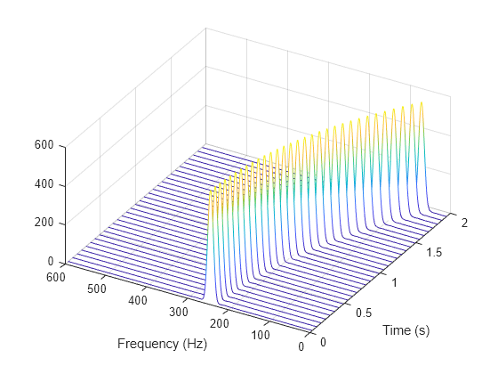
Generate a signal that consists of a complex-valued convex quadratic chirp sampled at 600 Hz for 2 seconds. The chirp has an initial frequency of 250 Hz and a final frequency of 50 Hz.

fs = 6e2; ts = 0:1/fs:2; x = chirp(ts,250,ts(end),50,"quadratic",0,"convex","complex");

spectrogram Function

Use the spectrogram function to compute the STFT of the signal.

Divide the signal into segments, each M=49 samples long.
Specify L=11 samples of overlap between adjoining segments.
Discard the final, shorter segment.
Window each segment with a Bartlett window.
Evaluate the discrete Fourier transform of each segment at NDFT=1024 points. By default, spectrogram computes two-sided transforms for complex-valued signals.

M = 49; L = 11; g = bartlett(M); Ndft = 1024;

[s,f,t] = spectrogram(x,g,L,Ndft,fs);

Use the waterplot function to compute and display the spectrogram, defined as the magnitude squared of the STFT.

Figure contains an axes object. The axes object with xlabel Frequency (Hz), ylabel Time (s) contains an object of type patch.

STFT Definition

Compute the STFT of the Nx-sample signal using the definition. Divide the signal into ⌊Nx-LM-L⌋ overlapping segments. Window each segment and evaluate its discrete Fourier transform at NDFT points.

segs = framesig(1:length(x),M,OverlapLength=L); X = fft(x(segs).*g,Ndft);

Compute the time and frequency ranges for the STFT.

To find the time values, divide the time vector into overlapping segments. The time values are the midpoints of the segments, with each segment treated as an interval open at the lower end.
To find the frequency values, specify a Nyquist interval closed at zero frequency and open at the lower end.

framedT = ts(segs); tint = mean(framedT(2:end,:));

fint = 0:fs/Ndft:fs-fs/Ndft;

Compare the output of spectrogram to the definition. Display the spectrogram.

maxdiff = max(max(abs(s-X)))

Figure contains an axes object. The axes object with xlabel Frequency (Hz), ylabel Time (s) contains an object of type patch.

function waterplot(s,f,t) % Waterfall plot of spectrogram waterfall(f,t,abs(s)'.^2) set(gca,XDir="reverse",View=[30 50]) xlabel("Frequency (Hz)") ylabel("Time (s)") end

Compare `spectrogram` and `stft` Functions

Generate a signal consisting of a chirp sampled at 1.4 kHz for 2 seconds. The frequency of the chirp decreases linearly from 600 Hz to 100 Hz during the measurement time.

fs = 1400; x = chirp(0:1/fs:2,600,2,100);

stft Defaults

Compute the STFT of the signal using the spectrogram and stft functions. Use the default values of the stft function:

Divide the signal into 128-sample segments and window each segment with a periodic Hann window.
Specify 96 samples of overlap between adjoining segments. This length is equivalent to 75% of the window length.
Specify 128 DFT points and center the STFT at zero frequency, with the frequency expressed in hertz.

Verify that the two results are equal.

M = 128; g = hann(M,"periodic"); L = 0.75*M; Ndft = 128;

[sp,fp,tp] = spectrogram(x,g,L,Ndft,fs,"centered");

[s,f,t] = stft(x,fs);

dff = max(max(abs(sp-s)))

Use the mesh function to plot the two outputs.

nexttile mesh(tp,fp,abs(sp).^2) title("spectrogram") view(2), axis tight

nexttile mesh(t,f,abs(s).^2) title("stft") view(2), axis tight

Figure contains 2 axes objects. Axes object 1 with title spectrogram contains an object of type surface. Axes object 2 with title stft contains an object of type surface.

spectrogram Defaults

Repeat the computation using the default values of the spectrogram function:

Divide the signal into segments of length M=⌊Nx/4.5⌋, where Nx is the length of the signal. Window each segment with a Hamming window.
Specify 50% overlap between segments.
To compute the FFT, use max(256,2⌈log2M⌉) points. Compute the spectrogram only for positive normalized frequencies.

M = floor(length(x)/4.5); g = hamming(M); L = floor(M/2); Ndft = max(256,2^nextpow2(M));

[sx,fx,tx] = spectrogram(x);

[st,ft,tt] = stft(x,Window=g,OverlapLength=L, ... FFTLength=Ndft,FrequencyRange="onesided");

dff = max(max(sx-st))

Use the waterplot function to plot the two outputs. Divide the frequency axis by π in both cases. For the stft output, divide the sample numbers by the effective sample rate, 2π.

figure nexttile waterplot(sx,fx/pi,tx) title("spectrogram")

nexttile waterplot(st,ft/pi,tt/(2*pi)) title("stft")

$Figure contains 2 axes objects. Axes object 1 with title spectrogram, xlabel Frequency/\pi, ylabel Samples contains an object of type patch. Axes object 2 with title stft, xlabel Frequency/\pi, ylabel Samples contains an object of type patch.$

function waterplot(s,f,t) % Waterfall plot of spectrogram waterfall(f,t,abs(s)'.^2) set(gca,XDir="reverse",View=[30 50]) xlabel("Frequency/\pi") ylabel("Samples") end

Compare `spectrogram` and `pspectrum` Functions

Generate a signal that consists of a voltage-controlled oscillator and three Gaussian atoms. The signal is sampled at fs=2 kHz for 2 seconds.

fs = 2000; tx = 0:1/fs:2; gaussFun = @(A,x,mu,f) exp(-(x-mu).^2/(20.03^2)).sin(2pif.*x)*A'; s = gaussFun([1 1 1],tx',[0.1 0.65 1],[2 6 2]*100)*1.5; x = vco(chirp(tx+.1,0,tx(end),3).exp(-2(tx-1).^2),[0.1 0.4]*fs,fs); x = s+x';

Short-Time Fourier Transforms

Use the pspectrum function to compute the STFT.

Divide the Nx-sample signal into segments of length M=80 samples, corresponding to a time resolution of 80/2000=40 milliseconds.
Specify L=16 samples or 20% of overlap between adjoining segments.
Window each segment with a Kaiser window and specify a leakage ℓ=0.7.

M = 80; L = 16; lk = 0.7;

[S,F,T] = pspectrum(x,fs,"spectrogram", ... TimeResolution=M/fs,OverlapPercent=L/M*100, ... Leakage=lk);

Compare to the result obtained with the spectrogram function.

Specify the window length and overlap directly in samples.
pspectrum always uses a Kaiser window as g(n). The leakage ℓ and the shape factor β of the window are related by β=40×(1-ℓ).
pspectrum always uses NDFT=1024 points when computing the discrete Fourier transform. You can specify this number if you want to compute the transform over a two-sided or centered frequency range. However, for one-sided transforms, which are the default for real signals, spectrogram uses 1024/2+1=513 points. Alternatively, you can specify the vector of frequencies at which you want to compute the transform, as in this example.
If a signal cannot be divided exactly into k=⌊Nx-LM-L⌋ segments, spectrogram truncates the signal whereas pspectrum pads the signal with zeros to create an extra segment. To make the outputs equivalent, remove the final segment and the final element of the time vector.
spectrogram returns the STFT, whose magnitude squared is the spectrogram. pspectrum returns the segment-by-segment power spectrum, which is already squared but is divided by a factor of ∑ng(n) before squaring.
For one-sided transforms, pspectrum adds an extra factor of 2 to the spectrogram.

g = kaiser(M,40*(1-lk));

k = (length(x)-L)/(M-L); if k~=floor(k) S = S(:,1:floor(k)); T = T(1:floor(k)); end

[s,f,t] = spectrogram(x/sum(g)*sqrt(2),g,L,F,fs);

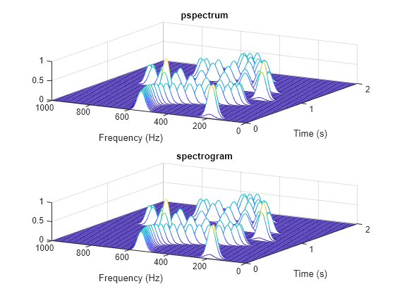
Use the waterplot function to display the spectrograms computed by the two functions.

subplot(2,1,1) waterplot(sqrt(S),F,T) title("pspectrum")

subplot(2,1,2) waterplot(s,f,t) title("spectrogram")

Figure contains 2 axes objects. Axes object 1 with title pspectrum, xlabel Frequency (Hz), ylabel Time (s) contains an object of type patch. Axes object 2 with title spectrogram, xlabel Frequency (Hz), ylabel Time (s) contains an object of type patch.

maxd = max(max(abs(abs(s).^2-S)))

Power Spectra and Convenience Plots

The spectrogram function has a fourth argument that corresponds to the segment-by-segment power spectrum or power spectral density. Similar to the output of pspectrum, the ps argument is already squared and includes the normalization factor ∑ng(n). For one-sided spectrograms of real signals, you still have to include the extra factor of 2. Set the scaling argument of the function to "power".

[,,~,ps] = spectrogram(x*sqrt(2),g,L,F,fs,"power");

max(abs(S(:)-ps(:)))

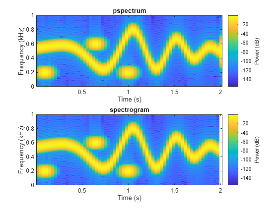
When called with no output arguments, both pspectrum and spectrogram plot the spectrogram of the signal in decibels. Include the factor of 2 for one-sided spectrograms. Set the colormaps to be the same for both plots. Set the _x_-limits to the same values to make visible the extra segment at the end of the pspectrum plot. In the spectrogram plot, display the frequency on the _y_-axis.

subplot(2,1,1) pspectrum(x,fs,"spectrogram", ... TimeResolution=M/fs,OverlapPercent=L/M*100, ... Leakage=lk) title("pspectrum") cc = clim; xl = xlim;

subplot(2,1,2) spectrogram(x*sqrt(2),g,L,F,fs,"power","yaxis") title("spectrogram") clim(cc) xlim(xl)

Figure contains 2 axes objects. Axes object 1 with title pspectrum, xlabel Time (s), ylabel Frequency (kHz) contains an object of type image. Axes object 2 with title spectrogram, xlabel Time (s), ylabel Frequency (kHz) contains an object of type image.

function waterplot(s,f,t) % Waterfall plot of spectrogram waterfall(f,t,abs(s)'.^2) set(gca,XDir="reverse",View=[30 50]) xlabel("Frequency (Hz)") ylabel("Time (s)") end

Compute Centered and One-Sided Spectrograms

Generate a signal that consists of a real-valued chirp sampled at 2 kHz for 2 seconds.

fs = 2000; tx = 0:1/fs:2; x = vco(-chirp(tx,0,tx(end),2).exp(-3(tx-1).^2), ... [0.1 0.4]*fs,fs).*hann(length(tx))';

Two-Sided Spectrogram

Compute and plot the two-sided STFT of the signal.

Divide the signal into segments, each M=73 samples long.
Specify L=24 samples of overlap between adjoining segments.
Discard the final, shorter segment.
Window each segment with a flat-top window.
Evaluate the discrete Fourier transform of each segment at NDFT=895 points, noting that it is an odd number.

M = 73; L = 24; g = flattopwin(M); Ndft = 895; neven = ~mod(Ndft,2);

[stwo,f,t] = spectrogram(x,g,L,Ndft,fs,"twosided");

Use the spectrogram function with no output arguments to plot the two-sided spectrogram.

spectrogram(x,g,L,Ndft,fs,"twosided","power","yaxis")

Figure contains an axes object. The axes object with xlabel Time (s), ylabel Frequency (kHz) contains an object of type image.

Compute the two-sided spectrogram using the definition. Divide the signal into M-sample segments with L samples of overlap between adjoining segments. Window each segment and compute its discrete Fourier transform at NDFT points.

y = framesig(x,M,Window=g,OverlapLength=L); Xtwo = fft(y,Ndft);

Compute the time and frequency ranges.

To find the time values, divide the time vector into overlapping segments. The time values are the midpoints of the segments, with each segment treated as an interval open at the lower end.
To find the frequency values, specify a Nyquist interval closed at zero frequency and open at the upper end.

framedT = framesig(tx,M,OverlapLength=L); ttwo = mean(framedT(2:end,:));

ftwo = 0:fs/Ndft:fs*(1-1/Ndft);

Compare the outputs of spectrogram to the definitions. Use the waterplot function to display the spectrograms.

diffs = [max(max(abs(stwo-Xtwo))); max(abs(f-ftwo')); max(abs(t-ttwo))]

diffs = 3×1 10-12 ×

     0
0.2274
0.0002

figure nexttile waterplot(Xtwo,ftwo,ttwo) title("Two-Sided, Definition")

nexttile waterplot(stwo,f,t) title("Two-Sided, spectrogram Function")

Figure contains 2 axes objects. Axes object 1 with title Two-Sided, Definition, xlabel Frequency (Hz), ylabel Time (s) contains an object of type patch. Axes object 2 with title Two-Sided, spectrogram Function, xlabel Frequency (Hz), ylabel Time (s) contains an object of type patch.

Centered Spectrogram

Compute the centered spectrogram of the signal.

Use the same time values that you used for the two-sided STFT.
Use the fftshift function to shift the zero-frequency component of the STFT to the center of the spectrum.
For odd-valued NDFT, the frequency interval is open at both ends. For even-valued NDFT, the frequency interval is open at the lower end and closed at the upper end.

Compare the outputs and display the spectrograms.

tcen = ttwo;

if ~neven Xcen = fftshift(Xtwo,1); fcen = -fs/2*(1-1/Ndft):fs/Ndft:fs/2; else Xcen = fftshift(circshift(Xtwo,-1),1); fcen = (-fs/2*(1-1/Ndft):fs/Ndft:fs/2)+fs/Ndft/2; end

[scen,f,t] = spectrogram(x,g,L,Ndft,fs,"centered");

diffs = [max(max(abs(scen-Xcen))); max(abs(f-fcen')); max(abs(t-tcen))]

diffs = 3×1 10-12 ×

     0
0.2274
0.0002

figure nexttile waterplot(Xcen,fcen,tcen) title("Centered, Definition")

nexttile waterplot(scen,f,t) title("Centered, spectrogram Function")

Figure contains 2 axes objects. Axes object 1 with title Centered, Definition, xlabel Frequency (Hz), ylabel Time (s) contains an object of type patch. Axes object 2 with title Centered, spectrogram Function, xlabel Frequency (Hz), ylabel Time (s) contains an object of type patch.

One-Sided Spectrogram

Compute the one-sided spectrogram of the signal.

Use the same time values that you used for the two-sided STFT.
For odd-valued NDFT, the one-sided STFT consists of the first (NDFT+1)/2 rows of the two-sided STFT. For even-valued NDFT, the one-sided STFT consists of the first NDFT/2+1 rows of the two-sided STFT.
For odd-valued NDFT, the frequency interval is closed at zero frequency and open at the Nyquist frequency. For even-valued NDFT, the frequency interval is closed at both ends.

Compare the outputs and display the spectrograms. For real-valued signals, the "onesided" argument is optional.

tone = ttwo;

if ~neven Xone = Xtwo(1:(Ndft+1)/2,:); else Xone = Xtwo(1:Ndft/2+1,:); end

fone = 0:fs/Ndft:fs/2;

[sone,f,t] = spectrogram(x,g,L,Ndft,fs);

diffs = [max(max(abs(sone-Xone))); max(abs(f-fone')); max(abs(t-tone))]

diffs = 3×1 10-12 ×

     0
0.1137
0.0002

figure nexttile waterplot(Xone,fone,tone) title("One-Sided, Definition")

nexttile waterplot(sone,f,t) title("One-Sided, spectrogram Function")

Figure contains 2 axes objects. Axes object 1 with title One-Sided, Definition, xlabel Frequency (Hz), ylabel Time (s) contains an object of type patch. Axes object 2 with title One-Sided, spectrogram Function, xlabel Frequency (Hz), ylabel Time (s) contains an object of type patch.

function waterplot(s,f,t) % Waterfall plot of spectrogram waterfall(f,t,abs(s)'.^2) set(gca,XDir="reverse",View=[30 50]) xlabel("Frequency (Hz)") ylabel("Time (s)") end

Compute Segment PSDs and Power Spectra

The spectrogram function has a matrix containing either the power spectral density (PSD) or the power spectrum of each segment as the fourth output argument. The power spectrum is equal to the PSD multiplied by the equivalent noise bandwidth (ENBW) of the window.

Generate a signal that consists of a logarithmic chirp sampled at 1 kHz for 1 second. The chirp has an initial frequency of 400 Hz that decreases to 10 Hz by the end of the measurement.

fs = 1000; tt = 0:1/fs:1-1/fs; y = chirp(tt,400,tt(end),10,"logarithmic");

Segment PSDs and Power Spectra with Sample Rate

Divide the signal into 102-sample segments and window each segment with a Hann window. Specify 12 samples of overlap between adjoining segments and 1024 DFT points.

M = 102; g = hann(M); L = 12; Ndft = 1024;

Compute the spectrogram of the signal with the default PSD spectrum type. Output the STFT and the array of segment power spectral densities.

[s,f,t,p] = spectrogram(y,g,L,Ndft,fs);

Repeat the computation with the spectrum type specified as "power". Output the STFT and the array of segment power spectra.

[r,,,q] = spectrogram(y,g,L,Ndft,fs,"power");

Verify that the spectrogram is the same in both cases. Plot the spectrogram using a logarithmic scale for the frequency.

max(max(abs(s).^2-abs(r).^2))

waterfall(f,t,abs(s)'.^2) set(gca,XScale="log",... XDir="reverse",View=[30 50])

Figure contains an axes object. The axes object contains an object of type patch.

Verify that the power spectra are equal to the power spectral densities multiplied by the ENBW of the window.

max(max(abs(q-p*enbw(g,fs))))

Verify that the matrix of segment power spectra is proportional to the spectrogram. The proportionality factor is the square of the sum of the window elements.

max(max(abs(s).^2-q*sum(g)^2))

Segment PSDs and Power Spectra with Normalized Frequencies

Repeat the computation, but now work in normalized frequencies. The results are the same when you specify the sample rate as 2π.

[,,~~,pn] = spectrogram(y,g,L,Ndft); [~~,,,qn] = spectrogram(y,g,L,Ndft,"power");

max(max(abs(qn-pnenbw(g,2pi))))

Spectrogram Computation with Signal Processing Toolbox - MATLAB & Simulink (original) (raw)

Functions for Spectrogram Computation

STFT and Spectrogram Definitions

Compare `spectrogram` Function and STFT Definition

Compare `spectrogram` and `stft` Functions

Compare `spectrogram` and `pspectrum` Functions

Compute Centered and One-Sided Spectrograms

Compute Segment PSDs and Power Spectra

See Also

Apps

Functions

Objects

Topics

External Websites

Spectrogram Computation with Signal Processing Toolbox - MATLAB & Simulink (original) (raw)

Functions for Spectrogram Computation

STFT and Spectrogram Definitions

Compare spectrogram Function and STFT Definition

Compare spectrogram and stft Functions

Compare spectrogram and pspectrum Functions

Compute Centered and One-Sided Spectrograms

Compute Segment PSDs and Power Spectra

See Also

Apps

Functions

Objects

Topics

External Websites

Compare `spectrogram` Function and STFT Definition

Compare `spectrogram` and `stft` Functions

Compare `spectrogram` and `pspectrum` Functions