importNetworkFromPyTorch - Import PyTorch network as MATLAB network - MATLAB (original) (raw)
Import PyTorch network as MATLAB network
Since R2022b
Syntax
Description
[net](#mw%5Feb57ebe8-0198-40e8-9ced-1da62482e14f) = importNetworkFromPyTorch([modelfile](#mw%5F5b3b9d1e-30ec-435a-a0cc-9dd86bbb76c8)) imports a pretrained and traced PyTorch® model from the file modelfile. The function returns the network net as an uninitialized dlnetwork object.
importNetworkFromPyTorch requires the Deep Learning Toolbox™ Converter for PyTorch Models support package. If this support package is not installed, thenimportNetworkFromPyTorch provides a download link.
Note
The importNetworkFromPyTorch function can generate a custom layer when you import a PyTorch layer. For more information, see Algorithms. The function saves the generated custom layers in the + modelfile namespace.
[net](#mw%5Feb57ebe8-0198-40e8-9ced-1da62482e14f) = importNetworkFromPyTorch([modelfile](#mw%5F5b3b9d1e-30ec-435a-a0cc-9dd86bbb76c8),[Name=Value](#namevaluepairarguments)) imports a pretrained and traced PyTorch network with additional options specified by one or more name-value arguments. For example, Namespace="CustomLayers" saves any generated custom layers and associated functions in the +CustomLayers namespace in the current folder. If the PyTorchInputSizes name-value argument is specified, then the function may return the network net as an initializeddlnetwork.
For information about how to trace a PyTorch model, see https://pytorch.org/docs/stable/generated/torch.jit.trace.html.
Examples
Import Network from PyTorch and Add Input Layer
Import a pretrained and traced PyTorch model as an uninitialized dlnetwork object. Then, add an input layer to the imported network.
This example imports the MNASNet (Copyright© Soumith Chintala 2016) PyTorch model. MNASNet is an image classification model that is trained with images from the ImageNet database. Download the mnasnet1_0 file, which is approximately 17 MB in size, from the MathWorks website.
modelfile = matlab.internal.examples.downloadSupportFile("nnet", ... "data/PyTorchModels/mnasnet1_0.pt");
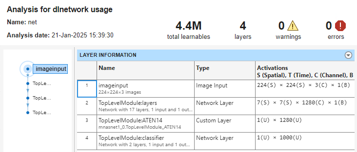
Import the MNASNet model by using the importNetworkFromPyTorch function. The function imports the model as an uninitialized dlnetwork object without an input layer. The software displays a warning that contains information about the number of input layers, what type of input layer to add, and how to add an input layer.
net = importNetworkFromPyTorch(modelfile)
Warning: Network was imported as an uninitialized dlnetwork. Before using the network, add input layer(s):
% Create imageInputLayer for the network input at index 1: inputLayer1 = imageInputLayer(, Normalization="none");
% Add input layers to the network and initialize: net = addInputLayer(net, inputLayer1, Initialize=true);
net = dlnetwork with properties:
     Layers: [1×1 nnet.cnn.layer.NetworkLayer]
Connections: [0×2 table]
 Learnables: [210×3 table]
      State: [104×3 table]
 InputNames: {'TopLevelModule'}
OutputNames: {'TopLevelModule'}
Initialized: 0
View summary with summary.
Specify the input size of the imported network and create an image input layer. Then, add the image input layer to the imported network and initialize the network by using the addInputLayer function.
InputSize = [224 224 3]; inputLayer = imageInputLayer(InputSize,Normalization="none"); net = addInputLayer(net,inputLayer,Initialize=true);
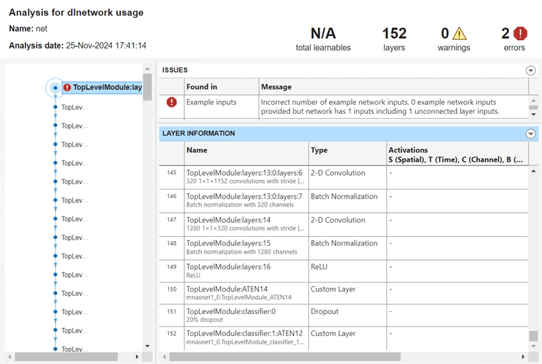
Analyze the imported network and view the input layer. The network is ready to use for prediction.
Import Network from PyTorch using PyTorchInputSizes
Import a pretrained and traced PyTorch model as an initialized dlnetwork object using the name-value argument PyTorchInputSizes.
This example imports the MNASNet (Copyright© Soumith Chintala 2016) PyTorch model. MNASNet is an image classification model that is trained with images from the ImageNet database. Download the mnasnet1_0.pt file, which is approximately 17 MB in size, from the MathWorks website.
modelfile = matlab.internal.examples.downloadSupportFile("nnet", ... "data/PyTorchModels/mnasnet1_0.pt");
Import the MNASNet model by using the importNetworkFromPyTorch function with the name-value argument PyTorchInputSizes. We know that a 224x224 color image is a valid input size for this PyTorch model. The software automatically creates and adds the input layer for a batch of images. This allows the network to be imported as an initialized network in one line of code.
net = importNetworkFromPyTorch(modelfile,PyTorchInputSizes=[NaN,3,224,224])
net = dlnetwork with properties:
     Layers: [2×1 nnet.cnn.layer.Layer]
Connections: [1×2 table]
 Learnables: [210×3 table]
      State: [104×3 table]
 InputNames: {'InputLayer1'}
OutputNames: {'TopLevelModule'}
Initialized: 1
View summary with summary.
The network is ready to use for prediction.
Import Network from PyTorch and Initialize
Import a pretrained and traced PyTorch model as an uninitialized dlnetwork object. Then, initialize the imported network.
This example imports the MNASNet (Copyright© Soumith Chintal 2016) PyTorch model. MNASNet is an image classification model that is trained with images from the ImageNet database. Download the mnasnet1_0 file, which is approximately 17 MB in size, from the MathWorks website.
modelfile = matlab.internal.examples.downloadSupportFile("nnet", ... "data/PyTorchModels/mnasnet1_0.pt");
Import the MNASNet model by using the importNetworkFromPyTorch function. The function imports the model as an uninitialized dlnetwork object.
net = importNetworkFromPyTorch(modelfile)
Warning: Network was imported as an uninitialized dlnetwork. Before using the network, add input layer(s):
% Create imageInputLayer for the network input at index 1: inputLayer1 = imageInputLayer(, Normalization="none");
% Add input layers to the network and initialize: net = addInputLayer(net, inputLayer1, Initialize=true);
net = dlnetwork with properties:
     Layers: [1×1 nnet.cnn.layer.NetworkLayer]
Connections: [0×2 table]
 Learnables: [210×3 table]
      State: [104×3 table]
 InputNames: {'TopLevelModule'}
OutputNames: {'TopLevelModule'}
Initialized: 0
View summary with summary.
net is a dlnetwork object consisting of a single networkLayer layer that contains a nested network. Specify the input size for net and create a random dlarray object that represents the input to the network. The data format of the dlarray object must have the dimensions "SSCB" (spatial, spatial, channel, batch) to represent a 2-D image input. For more information, see Data Formats for Prediction with dlnetwork.
InputSize = [224 224 3]; X = dlarray(rand(InputSize),"SSCB");
Initialize the learnable parameters of the imported network by using the initialize function.
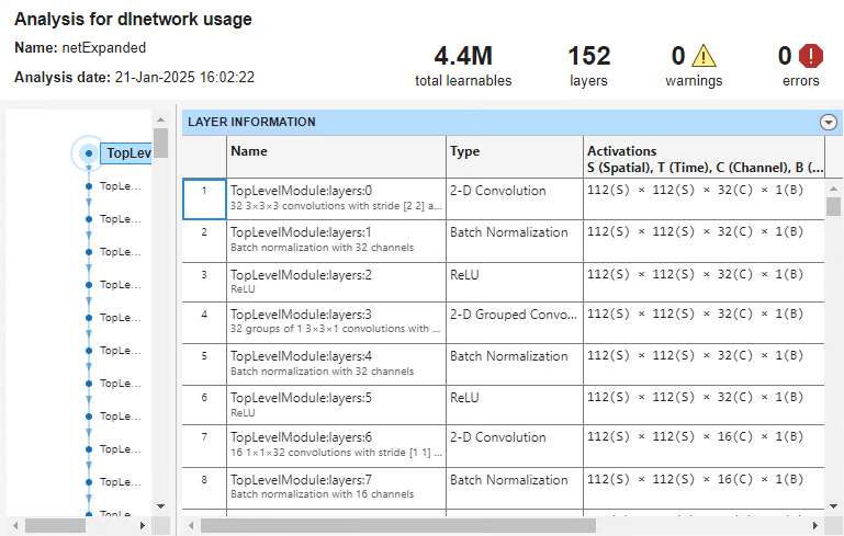
Now the imported network is ready to use for prediction. Expand the networkLayer using the expandLayers function and analyze the imported network.
netExpanded = expandLayers(net)
netExpanded = dlnetwork with properties:
     Layers: [152×1 nnet.cnn.layer.Layer]
Connections: [161×2 table]
 Learnables: [210×3 table]
      State: [104×3 table]
 InputNames: {'TopLevelModule:layers:0'}
OutputNames: {'TopLevelModule:classifier:1'}
Initialized: 1
View summary with summary.
analyzeNetwork(netExpanded)
Import Network from PyTorch and Classify Image
Import a pretrained and traced PyTorch model as an uninitialized dlnetwork object to classify an image.
This example imports the MNASNet (Copyright© Soumith Chintala 2016) PyTorch model. MNASNet is an image classification model that is trained with images from the ImageNet database. Download the mnasnet1_0 file, which is approximately 17 MB in size, from the MathWorks website.
modelfile = matlab.internal.examples.downloadSupportFile("nnet", ... "data/PyTorchModels/mnasnet1_0.pt");
Import the MNASNet model by using the importNetworkFromPyTorch function. The function imports the model as an uninitialized dlnetwork object.
net = importNetworkFromPyTorch(modelfile)
Warning: Network was imported as an uninitialized dlnetwork. Before using the network, add input layer(s):
% Create imageInputLayer for the network input at index 1: inputLayer1 = imageInputLayer(, Normalization="none");
% Add input layers to the network and initialize: net = addInputLayer(net, inputLayer1, Initialize=true);
net = dlnetwork with properties:
     Layers: [1×1 nnet.cnn.layer.NetworkLayer]
Connections: [0×2 table]
 Learnables: [210×3 table]
      State: [104×3 table]
 InputNames: {'TopLevelModule'}
OutputNames: {'TopLevelModule'}
Initialized: 0
View summary with summary.
Specify the input size of the imported network and create an image input layer. Then, add the image input layer to the imported network and initialize the network by using the addInputLayer function.
InputSize = [224 224 3]; inputLayer = imageInputLayer(InputSize,Normalization="none"); net = addInputLayer(net,inputLayer,Initialize=true);
Read the image you want to classify.
Im = imread("peppers.png");
Resize the image to the input size of the network. Show the image.
InputSize = [224 224 3]; Im = imresize(Im,InputSize(1:2)); imshow(Im)
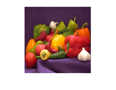
The inputs to MNASNet require further preprocessing. Rescale the image. Then, normalize the image by subtracting the training images mean and dividing by the training images standard deviation. For more information, see Input Data Preprocessing.
Im = rescale(Im,0,1);
meanIm = [0.485 0.456 0.406]; stdIm = [0.229 0.224 0.225]; Im = (Im - reshape(meanIm,[1 1 3]))./reshape(stdIm,[1 1 3]);
Convert the image to a dlarray object. Format the image with the dimensions "SSCB" (spatial, spatial, channel, batch).
Im_dlarray = dlarray(single(Im),"SSCB");
Get the class names from squeezenet, which is also trained with ImageNet images.
[~,ClassNames] = imagePretrainedNetwork("squeezenet");
Classify the image and find the predicted label.
prob = predict(net,Im_dlarray); [~,label_ind] = max(prob);
Display the classification result.
Import Network from PyTorch and Find Generated Custom Layers
Import a pretrained and traced PyTorch model as an uninitialized dlnetwork object. Then, find the custom layers that the software generates.
This example uses the findCustomLayers helper function.
This example imports the MNASNet (Copyright© Soumith Chintala 2016) PyTorch model. MNASNet is an image classification model that is trained with images from the ImageNet database. Download the mnasnet1_0 file, which is approximately 17 MB in size, from the MathWorks website.
modelfile = matlab.internal.examples.downloadSupportFile("nnet", ... "data/PyTorchModels/mnasnet1_0.pt");
Import the MNASNet model by using the importNetworkFromPyTorch function. The function imports the model as an uninitialized dlnetwork object.
net = importNetworkFromPyTorch(modelfile)
Warning: Network was imported as an uninitialized dlnetwork. Before using the network, add input layer(s):
% Create imageInputLayer for the network input at index 1: inputLayer1 = imageInputLayer(, Normalization="none");
% Add input layers to the network and initialize: net = addInputLayer(net, inputLayer1, Initialize=true);
net = dlnetwork with properties:
     Layers: [1×1 nnet.cnn.layer.NetworkLayer]
Connections: [0×2 table]
 Learnables: [210×3 table]
      State: [104×3 table]
 InputNames: {'TopLevelModule'}
OutputNames: {'TopLevelModule'}
Initialized: 0
View summary with summary.
net is a dlnetwork object consisting of a single networkLayer layer that contains a nested network. Expand the nested network layers using the expandLayers function.
The importNetworkFromPyTorch function generates custom layers for the PyTorch layers that the function cannot convert to built-in MATLAB layers or functions. For more information, see Algorithms. The software saves the automatically generated custom layers to the +mnasnet1_0 namespace in the current folder and the associated functions to the +ops inner namespace. To see the custom layers and associated functions, inspect the namespace.
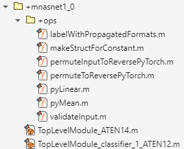
You can also find the indices of the generated custom layers by using the findCustomLayers helper function. Display the custom layers.
ind = findCustomLayers(net.Layers,'+mnasnet1_0'); net.Layers(ind)
ans = 13×1 Layer array with layers:
 1   'TopLevelModule:layers:0'              2-D Convolution           32 3×3×3 convolutions with stride [2  2] and padding [1  1  1  1]
 2   'TopLevelModule:layers:1'              Batch Normalization       Batch normalization with 32 channels
 3   'TopLevelModule:layers:2'              ReLU                      ReLU
 4   'TopLevelModule:layers:3'              2-D Grouped Convolution   32 groups of 1 3×3×1 convolutions with stride [1  1] and padding [1  1  1  1]
 5   'TopLevelModule:layers:4'              Batch Normalization       Batch normalization with 32 channels
 6   'TopLevelModule:layers:5'              ReLU                      ReLU
 7   'TopLevelModule:layers:6'              2-D Convolution           16 1×1×32 convolutions with stride [1  1] and padding [0  0  0  0]
 8   'TopLevelModule:layers:7'              Batch Normalization       Batch normalization with 16 channels
 9   'TopLevelModule:layers:8:0:layers:0'   2-D Convolution           48 1×1×16 convolutions with stride [1  1] and padding [0  0  0  0]
10   'TopLevelModule:layers:8:0:layers:1'   Batch Normalization       Batch normalization with 48 channels
11   'TopLevelModule:layers:8:0:layers:2'   ReLU                      ReLU
12   'TopLevelModule:layers:8:0:layers:6'   2-D Convolution           24 1×1×48 convolutions with stride [1  1] and padding [0  0  0  0]
13 'TopLevelModule:layers:8:0:layers:7' Batch Normalization Batch normalization with 24 channels**Helper Function
The findCustomLayers helper function returns a logical vector corresponding to the indices of the custom layers that importNetworkFromPyTorch automatically generates.
function indices = findCustomLayers(layers,Namespace)
s = what(['.' filesep Namespace]);
indices = zeros(1,length(s.m)); for i = 1:length(layers) for j = 1:length(s.m) if strcmpi(class(layers(i)),[Namespace(2:end) '.' s.m{j}(1:end-2)]) indices(j) = i; end end indices = logical(indices); end
end
Train Network Imported from PyTorch to Classify New Images
This example shows how to import a network from PyTorch and train the network to classify new images. Use the importNetworkFromPytorch function to import the network as an uninitialized dlnetwork object. Train the network by using a custom training loop.
This example uses the modelLoss, modelPredictions, and preprocessMiniBatchPredictors helper functions.
This example also uses the supporting file new_fcLayer. To access the supporting file, open the example in Live Editor.
**Load Data
Unzip the MerchData data set, which contains 75 images. Load the new images as an image datastore. The imageDatastore function automatically labels the images based on folder names and stores the data as an ImageDatastore object. Divide the data into training and validation data sets. Use 70% of the images for training and 30% for validation.
unzip("MerchData.zip"); imds = imageDatastore("MerchData", ... IncludeSubfolders=true, ... LabelSource="foldernames"); [imdsTrain,imdsValidation] = splitEachLabel(imds,0.7);
The network you use in this example requires input images with a size of 224-by-224-by-3. To automatically resize the training images, use an augmented image datastore. Randomly translate the images up to 30 pixels in the horizontal and vertical axes. Data augmentation helps prevent the network from overfitting and memorizing the exact details of the training images.
inputSize = [224 224 3];
pixelRange = [-30 30]; scaleRange = [0.9 1.1]; imageAugmenter = imageDataAugmenter(... RandXReflection=true, ... RandXTranslation=pixelRange, ... RandYTranslation=pixelRange, ... RandXScale=scaleRange, ... RandYScale=scaleRange); augimdsTrain = augmentedImageDatastore(inputSize(1:2),imdsTrain, ... DataAugmentation=imageAugmenter);
To automatically resize the validation images without performing further data augmentation, use an augmented image datastore without specifying any additional preprocessing operations.
augimdsValidation = augmentedImageDatastore(inputSize(1:2),imdsValidation);
Determine the number of classes in the training data.
classes = categories(imdsTrain.Labels); numClasses = numel(classes);
**Import Network
Download the MNASNet (Copyright© Soumith Chintala 2016) PyTorch model. MNASNet is an image classification model that is trained with images from the ImageNet database. Download the mnasnet1_0 file, which is approximately 17 MB in size, from the MathWorks website.
modelfile = matlab.internal.examples.downloadSupportFile("nnet", ... "data/PyTorchModels/mnasnet1_0.pt");
Import the MNASNet model as an uninitialized dlnetwork object by using the importNetworkFromPyTorch function.
net = importNetworkFromPyTorch(modelfile)
Warning: Network was imported as an uninitialized dlnetwork. Before using the network, add input layer(s):
% Create imageInputLayer for the network input at index 1: inputLayer1 = imageInputLayer(, Normalization="none");
% Add input layers to the network and initialize: net = addInputLayer(net, inputLayer1, Initialize=true);
net = dlnetwork with properties:
     Layers: [1×1 nnet.cnn.layer.NetworkLayer]
Connections: [0×2 table]
 Learnables: [210×3 table]
      State: [104×3 table]
 InputNames: {'TopLevelModule'}
OutputNames: {'TopLevelModule'}
Initialized: 0
View summary with summary.
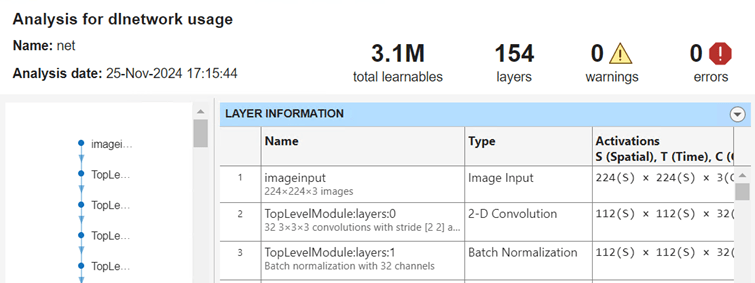
net is a dlnetwork object consisting of a single networkLayer layer that contains a nested network. Expand the networkLayer using the expandLayers function. Display the final layer of the imported network using the analyzeNetwork function.
net = expandLayers(net); analyzeNetwork(net)
The TopLevelModule:classifier:1 layer is a custom layer generated by the importNetworkFromPyTorch function and the last learnable layer of the imported network. This layer contains information about how to combine the features that the network extracts into class probabilities and a loss value.
Replace Final Layer
To retrain the imported network to classify new images, replace the final layers with a new fully connected layer. The new layer new_fclayer is adapted to the new data set and must also be a custom layer because it has two inputs.
Initialize the new_fcLayer layer and replace the TopLevelModule:classifier:1 layer with new_fcLayer.
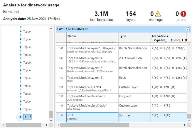
newLayer = new_fcLayer("TopLevelModule:classifier:fc1","Custom Layer", ... {'in'},{'out'},numClasses); net = replaceLayer(net,"TopLevelModule:classifier:1",newLayer);
Add a softmax layer to the network and connect the softmax layer to the new fully connected layer.
net = addLayers(net,softmaxLayer(Name="sm1")); net = connectLayers(net,"TopLevelModule:classifier:fc1","sm1");
Add Input Layer
Add an image input layer to the network and initialize the network.
inputLayer = imageInputLayer(inputSize,Normalization="none"); net = addInputLayer(net,inputLayer,Initialize=true);
Analyze the network. View the first layer and the final layers.
Define Model Loss Function
Training a deep neural network is an optimization task. By treating a neural network as a function f(X;θ), where X is the network input and θ is the set of learnable parameters, you can optimize θ so that it minimizes some loss value based on the training data. For example, optimize the learnable parameters θ such that, for inputs X with corresponding targets T, they minimize the error between the predictions Y=f(X;θ) and T.
Create the modelLoss function, listed in the Model Loss Function section of the example, which takes as input the dlnetwork object and a mini-batch of input data with corresponding targets. The function returns the loss, the gradients of the loss with respect to the learnable parameters, and the network state.
Specify Training Options
Train for 15 epochs with a mini-batch size of 20.
numEpochs = 15; miniBatchSize = 20;
Specify the options for SGDM optimization. Specify an initial learning rate of 0.001 with a decay of 0.005, and a momentum of 0.9.
initialLearnRate = 0.001; decay = 0.005; momentum = 0.9;
Train Network
Create a minibatchqueue object that processes and manages mini-batches of images during training. For each mini-batch, perform these steps:
- Use the custom mini-batch preprocessing function
preprocessMiniBatch(defined at the end of this example) to convert the labels to one-hot encoded variables. - Format the image data with the dimension labels
"SSCB"(spatial, spatial, channel, batch). By default, theminibatchqueueobject converts the data todlarrayobjects with the underlying typesingle. Do not format the class labels. - Train on a GPU if one is available. By default, the
minibatchqueueobject converts each output to agpuArrayobject if a GPU is available. Using a GPU requires a Parallel Computing Toolbox™ license and a supported GPU device. For information about supported devices, see GPU Computing Requirements (Parallel Computing Toolbox).
mbq = minibatchqueue(augimdsTrain,... MiniBatchSize=miniBatchSize,... MiniBatchFcn=@preprocessMiniBatch,... MiniBatchFormat=["SSCB" ""]);
Initialize the velocity parameter for the gradient descent with momentum (SGDM) solver.
Calculate the total number of iterations for the training progress monitor.
numObservationsTrain = numel(imdsTrain.Files); numIterationsPerEpoch = ceil(numObservationsTrain/miniBatchSize); numIterations = numEpochs*numIterationsPerEpoch;
Initialize the trainingProgressMonitor object. Because the timer starts when you create the monitor object, create the object immediately after the training loop.
monitor = trainingProgressMonitor(Metrics="Loss",Info=["Epoch","LearnRate"],XLabel="Iteration");
Train the network using a custom training loop. For each epoch, shuffle the data and loop over mini-batches of data. For each mini-batch, perform these steps:
- Evaluate the model loss, gradients, and state using the dlfeval and modelLoss functions and then update the network state.
- Determine the learning rate for the time-based decay learning rate schedule.
- Update the network parameters using the sgdmupdate function.
- Update the loss, learning rate, and epoch values in the training progress monitor.
- Stop if the
Stopproperty is true. TheStopproperty value of theTrainingProgressMonitorobject changes totruewhen you click the Stop button.
epoch = 0; iteration = 0;
% Loop over epochs. while epoch < numEpochs && ~monitor.Stop
epoch = epoch + 1;

% Shuffle data.
shuffle(mbq);

% Loop over mini-batches.
while hasdata(mbq) && ~monitor.Stop

    iteration = iteration + 1;

    % Read mini-batch of data.
    [X,T] = next(mbq);

    % Evaluate the model gradients, state, and loss using dlfeval and the
    % modelLoss function and update the network state.
    [loss,gradients,state] = dlfeval(@modelLoss,net,X,T);
    net.State = state;

    % Determine learning rate for time-based decay learning rate schedule.
    learnRate = initialLearnRate/(1 + decay*iteration);

    % Update the network parameters using the SGDM optimizer.
    [net,velocity] = sgdmupdate(net,gradients,velocity,learnRate,momentum);

    % Update the training progress monitor.
    recordMetrics(monitor,iteration,Loss=loss);
    updateInfo(monitor,Epoch=epoch,LearnRate=learnRate);
    monitor.Progress = 100*iteration/numIterations;
end
end

Classify Validation Images
Test the classification accuracy of the model by comparing the predictions on the validation set with the true labels.
After training, making predictions on new data does not require the labels. Create a minibatchqueue object containing only the predictors of the test data:
- To ignore the labels for testing, set the number of outputs of the mini-batch queue to 1.
- Specify the same mini-batch size that you use for training.
- Preprocess the predictors using the
preprocessMiniBatchPredictorsfunction, listed at the end of the example. - For the single output of the datastore, specify the mini-batch format
"SSCB"(spatial, spatial, channel, batch).
numOutputs = 1;
mbqTest = minibatchqueue(augimdsValidation,numOutputs, ... MiniBatchSize=miniBatchSize, ... MiniBatchFcn=@preprocessMiniBatchPredictors, ... MiniBatchFormat="SSCB");
Loop over the mini-batches and classify the images using the modelPredictions function, listed at the end of the example.
YTest = modelPredictions(net,mbqTest,classes);
Evaluate the classification accuracy.
TTest = imdsValidation.Labels; accuracy = mean(TTest == YTest)
Visualize the predictions in a confusion chart. Large values on the diagonal indicate accurate predictions for the corresponding class. Large values on the off-diagonal indicate strong confusion between the corresponding classes.
figure confusionchart(TTest,YTest)

Helper Functions
Model Loss Function
The modelLoss function takes as input a dlnetwork object net and a mini-batch of input data X with corresponding targets T. The function returns the loss, the gradients of the loss with respect to the learnable parameters in net, and the network state. To compute the gradients automatically, use the dlgradient function.
function [loss,gradients,state] = modelLoss(net,X,T)
% Forward data through network. [Y,state] = forward(net,X);
% Calculate cross-entropy loss. loss = crossentropy(Y,T);
% Calculate gradients of loss with respect to learnable parameters. gradients = dlgradient(loss,net.Learnables);
end
Model Predictions Function
The modelPredictions function takes as input a dlnetwork object net, a minibatchqueue of input data mbq, and the network classes. The function computes the model predictions by iterating over all the data in the minibatchqueue object. The function uses the onehotdecode function to find the predicted class with the highest score.
function Y = modelPredictions(net,mbq,classes)
Y = [];
% Loop over mini-batches. while hasdata(mbq) X = next(mbq);
% Make prediction.
scores = predict(net,X);

% Decode labels and append to output.
labels = onehotdecode(scores,classes,1)';
Y = [Y; labels];
end
end
Mini Batch Preprocessing Function
The preprocessMiniBatch function preprocesses a mini-batch of predictors and labels using these steps:
- Preprocess the images using the
preprocessMiniBatchPredictorsfunction. - Extract the label data from the incoming cell array and concatenate the result into a categorical array along the second dimension.
- One-hot encode the categorical labels into numeric arrays. Encoding into the first dimension produces an encoded array that matches the shape of the network output.
function [X,T] = preprocessMiniBatch(dataX,dataT)
% Preprocess predictors. X = preprocessMiniBatchPredictors(dataX);
% Extract label data from cell and concatenate. T = cat(2,dataT{1:end});
% One-hot encode labels. T = onehotencode(T,1);
end
Mini-Batch Predictors Preprocessing Function
The preprocessMiniBatchPredictors function preprocesses a mini-batch of predictors by extracting the image data from the input cell array and concatenating the result into a numeric array. For grayscale input, concatenating over the fourth dimension adds a third dimension to each image to use as a singleton channel dimension.
function X = preprocessMiniBatchPredictors(dataX)
% Concatenate. X = cat(4,dataX{1:end});
end
Input Arguments
modelfile — Name of PyTorch model file
character vector | string scalar
Name of the PyTorch model file, specified as a character vector or string scalar.modelfile must be in the current folder, or you must include a full or relative path to the file. The PyTorch model must be pretrained and traced over one inference iteration.
For information about how to trace a PyTorch model, see https://pytorch.org/docs/stable/generated/torch.jit.trace.html.
Example: "mobilenet_v3.pt"
Name-Value Arguments
Specify optional pairs of arguments asName1=Value1,...,NameN=ValueN, where Name is the argument name and Value is the corresponding value. Name-value arguments must appear after other arguments, but the order of the pairs does not matter.
Example: importNetworkFromPyTorch(modelfile,Namespace="CustomLayers") imports the network in modelfile and saves the custom layers namespace+`Namespace` in the current folder.
Namespace — Name of custom layers namespace
character vector | string scalar
Name of the custom layers namespace in which importNetworkFromPyTorch saves custom layers, specified as a character vector or string scalar.importNetworkFromPyTorch saves the custom layers+`Namespace` namespace in the current folder. If you do not specify Namespace, thenimportNetworkFromPyTorch saves the custom layers in the+[modelfile](#mw%5F5b3b9d1e-30ec-435a-a0cc-9dd86bbb76c8) namespace in the current folder. For more information about namespaces, see Create Namespaces.
importNetworkFromPyTorch tries to generate a custom layer when you import a custom PyTorch layer or when the software cannot convert a PyTorch layer into an equivalent built-in MATLAB® layer. importNetworkFromPyTorch saves each generated custom layer to a separate MATLAB code file in +`Namespace`. To view or edit a custom layer, open the associated MATLAB code file. For more information about custom layers, see Custom Layers.
The +`Namespace` namespace can also contain the +ops inner namespace. This inner namespace contains MATLAB functions corresponding to PyTorch operators that the automatically generated custom layers use.importNetworkFromPyTorch saves the associated MATLAB function for each operator in a separate MATLAB code file in the +ops inner namespace. The object functions of dlnetwork, such as the predict function, use these operators when it interacts with the custom layers. The +ops inner namespace can also contain placeholder functions. For more information, seePlaceholder Functions.
Example: Namespace="mobilenet_v3"
PyTorchInputSizes — Dimension sizes of network inputs
numeric array | string scalar | cell array
Dimension sizes of the PyTorch network inputs, specified as a numeric array, string scalar, or cell array. The dimension input order is the same as in the PyTorch network. You can specify PyTorchInputSizes as a numeric array only when the network has a single nonscalar input. If the network has multiple inputs, PyTorchInputSizes must be a cell array of the input sizes. For an input whose size or shape is not known specifyPyTorchInputSize as "unknown". For an input that corresponds to a 0-dimensional scalar in PyTorch, specify PyTorchInputSize as"scalar".
The standard input layers that importNetworkFromPyTorch supports areImageInputLayer (SSCB), FeatureInputLayer (CB), ImageInputLayer3D (SSSCB), andSequenceInputLayer (CBT). Here, S is spatial, C is channel, B is batch, and T is time. importNetworkFromPyTorch also supports nonstandard inputs using PyTorchInputSizes. For example, import the network and specify the input dimension sizes with this function call: net = importNetworkFromPyTorch("nonStandardModel.pt",PyTorchInputSizes=[1 3 224]). Then, initialize the network with a U-labelleddlarray object, where U is unknown, with these function calls:X = dlarray(rand(1 3 224),"UUU") and net = initialize(net,X). The software interprets the U-labelleddlarray as data in PyTorch order.
Example: PyTorchInputSizes=[NaN 3 224 224] is a network with one input that is a batch of images.
Example: PyTorchInputSizes={[NaN 3 224 224],"unknown"} is a network with two inputs. The first input is a batch of images and the second input has unknown size.
Data Types: numeric array | string | cell array
PreferredNestingType — Network composition representation
"networklayer" (default) | "customlayer"
Network composition representation, specified as one of the following values:
"networklayer"— Represents network composition in the imported network using networkLayer layer objects."customlayer"— Represents network composition in the imported network using nested custom layers. For more information about custom layers, see Define Custom Deep Learning Layers.
Example: PreferredNestingType="customlayer"
Data Types: char | string
Output Arguments
Limitations
- The
importNetworkFromPyTorchfunction fully supports PyTorch version 2.0. The function can import most models created in other PyTorch versions. - The
importNetworkFromPyTorchfunction can import only image classification and segmentation models.
More About
Conversion of PyTorch Layers and Functions into Built-In MATLAB Layers and Functions
The importNetworkFromPyTorch function supports the PyTorch layers, functions, and operators listed in this section for conversion into built-in MATLAB layers and functions with dlarray support. For more information about functions that operate on dlarray objects, seeList of Functions with dlarray Support. The conversion process often has limitations.
Conversion of PyTorch Layers
This table shows the correspondence between PyTorch layers and Deep Learning Toolbox layers. In some cases, when importNetworkFromPyTorch cannot convert a PyTorch layer into a MATLAB layer, the software converts the PyTorch layer into a Deep Learning Toolbox function with dlarray support.
Conversion of PyTorch Functions
This table shows the correspondence between PyTorch functions and Deep Learning Toolbox functions.
| PyTorch Function | Corresponding Deep Learning Toolbox Function |
|---|---|
| torch.nn.functional.adaptive_avg_pool2d | pyAdaptiveAvgPool2d |
| torch.nn.functional.avg_pool2d | pyAvgPool2d |
| torch.nn.functional.conv1d | pyConvolution |
| torch.nn.functional.conv2d | pyConvolution |
| torch.nn.functional.dropout | pyDropout |
| torch.nn.functional.embedding | pyEmbedding |
| torch.nn.functional.gelu | pyGelu |
| torch.nn.functional.glu | pyGLU |
| torch.nn.functional.hardsigmoid | pyHardSigmoid |
| torch.nn.functional.hardswish | pyHardSwish |
| torch.nn.functional.layer_norm | pyLayerNorm |
| torch.nn.functional.leaky_relu | pyLeakyRelu |
| torch.nn.functional.linear | pyLinear |
| torch.nn.functional.log_softmax | pyLogSoftmax |
| torch.nn.functional.pad | pyPad |
| torch.nn.functional.max_pool2d | pyMaxPool2d |
| torch.nn.functional.relu | relu |
| torch.nn.functional.silu | pySilu |
| torch.nn.functional.softmax | pySoftmax |
| torch.nn.functional.tanh | tanh |
Conversion of PyTorch Mathematical Operators
This table shows the correspondence between PyTorch mathematical operators and Deep Learning Toolbox functions. The importNetworkFromPyTorch first tries to convert thecat PyTorch operator to a concatenation layer, then to a function.
| PyTorch Operator | Corresponding Deep Learning Toolbox Layer or Function | Alternative Deep Learning Toolbox Function |
|---|---|---|
| +, -, / | pyElementwiseBinary | Not applicable |
| torch.abs | pyAbs | Not applicable |
| torch.arange | pyArange | Not applicable |
| torch.argmax | pyArgMax | Not applicable |
| torch.baddbmm | pyBaddbmm | Not applicable |
| torch.bitwise_not | pyBitwiseNot | No applicable |
| torch.bmm | pyMatMul | Not applicable |
| torch.cat | concatenationLayer | pyConcat |
| torch.chunk | pyChunk | Not applicable |
| torch.clamp_min | pyClampMin | Not applicable |
| torch.clone | identityLayer | Not applicable |
| torch.concat | pyConcat | Not applicable |
| torch.cos | pyCos | Not applicable |
| torch.cumsum | pyCumsum | Not applicable |
| torch.detach | pyDetach | Not applicable |
| torch.eq | pyEq | Not applicable |
| torch.floor_div | pyElementwiseBinary | Not applicable |
| torch.gather | pyGather | Not applicable |
| torch.ge | pyGe | Not applicable |
| torch.matmul | pyMatMul | Not applicable |
| torch.max | pyMaxBinary/pyMaxUnary | Not applicable |
| torch.mean | pyMean | Not applicable |
| torch.mul, * | multiplicationLayer | pyElementwiseBinary |
| torch.norm | pyNorm | Not applicable |
| torch.permute | pyPermute | Not applicable |
| torch.pow | pyElementwiseBinary | Not applicable |
| torch.remainder | pyRemainder | Not applicable |
| torch.repeat | pyRepeat | Not applicable |
| torch.repeat_interleave | pyRepeatInterleave | Not applicable |
| torch.reshape | pyView | Not applicable |
| torch.rsqrt | pyRsqrt | Not applicable |
| torch.size | pySize | Not applicable |
| torch.sin | pySin | Not applicable |
| torch.split | pySplitWithSizes | Not applicable |
| torch.sqrt | pyElementwiseBinary | Not applicable |
| torch.square | pySquare | Not applicable |
| torch.squeeze | pySqueeze | Not applicable |
| torch.stack | pyStack | Not applicable |
| torch.sum | pySum | Not applicable |
| torch.t | pyT | Not applicable |
| torch.to | pyTo | Not applicable |
| torch.transpose | pyTranspose | Not applicable |
| torch.unsqueeze | pyUnsqueeze | Not applicable |
| torch.zeros | pyZeros | Not applicable |
| torch.zeros_like | pyZerosLike | Not applicable |
Conversion of PyTorch Matrix Operators
This table shows the correspondence between PyTorch matrix operators and Deep Learning Toolbox functions.
| PyTorch Operator | Corresponding Deep Learning Toolbox Function or Operator |
|---|---|
| Indexing (for example, X[:,1]) | pySlice |
| torch.tensor.contiguous | = |
| torch.tensor.expand | pyExpand |
| torch.tensor.expand_as | pyExpandAs |
| torch.tensor.masked_fill | pyMaskedFill |
| torch.tensor.select | pySlice |
| torch.tensor.view | pyView |
Placeholder Functions
When the importNetworkFromPyTorch function cannot convert a PyTorch layer into a built-in MATLAB layer or generate a custom layer with associated MATLAB functions, the function creates a custom layer with a placeholder function. You must complete the placeholder function before you can use the network.
This code snippet defines a custom layer with thepyAtenUnsupportedOperator placeholder function.
classdef UnsupportedOperator < nnet.layer.Layer
function [output] = predict(obj,arg1) % Placeholder function for aten:: output= pyAtenUnsupportedOperator(arg1,params); end
end
Tips
- To use a pretrained network for prediction or transfer learning on new images, you must preprocess your images in the same way as the images that you use to train the imported model. The most common preprocessing steps are resizing images, subtracting image average values, and converting the images from BGR format to RGB format.
- To resize images, use imresize. For example,
imresize(image,[227 227 3]). - To convert images from RGB to BGR format, use flip. For example,
flip(image,3).
For more information about preprocessing images for training and prediction, see Preprocess Images for Deep Learning.
- To resize images, use imresize. For example,
- The members of the
+[Namespace](#mw%5F6add0260-5570-46b9-afda-d6416d2f0c78)namespace are not accessible if the namespace parent folder is not on the MATLAB path. For more information, see Namespaces and the MATLAB Path. - MATLAB uses one-based indexing, whereas Python® uses zero-based indexing. In other words, the first element in an array has an index of 1 and 0 in MATLAB and Python, respectively. For more information about MATLAB indexing, see Array Indexing. In MATLAB, to use an array of indices (
ind) created in Python, convert the array toind+1. - If you encounter a Python library conflict, use the pyenv function to specify the
ExecutionModename-value argument as"OutOfProcess". - For more tips, see Tips on Importing Models from TensorFlow, PyTorch, and ONNX.
Algorithms
The importNetworkFromPyTorch function imports a PyTorch layer into MATLAB by trying these steps in order:
- The function tries to import the PyTorch layer as a built-in MATLAB layer. For more information, see Conversion of PyTorch Layers.
- The function tries to import the PyTorch layer as a built-in MATLAB function. For more information, see Conversion of PyTorch Layers.
- The function tries to import the PyTorch layer as a custom layer.
importNetworkFromPyTorchsaves the generated custom layers and the associated functions in the+[Namespace](#mw%5F6add0260-5570-46b9-afda-d6416d2f0c78)namespace. For an example, seeImport Network from PyTorch and Find Generated Custom Layers. - The function imports the PyTorch layer as a custom layer with a placeholder function. You must complete the placeholder function before you can use the network, see Placeholder Functions.
In the first three cases, the imported network is ready for prediction after you initialize it.
Alternative Functionality
App
You can also import models from external platforms using the Deep Network Designer app. The app uses the importNetworkFromPyTorch function to import the network. On import, the app shows an import report with details about any issues that require attention.
Version History
Introduced in R2022b
R2024b: Represent network composition using networkLayer
You can import a network that uses networkLayer objects to represent network composition. To specify whether the imported network represents composition using networkLayer or custom layer objects, use thePreferredNestingType name-value argument. For more information, seeDeep Learning Network Composition.
R2024b: Import networks with new layers, operators, and functions
You can import the following PyTorch operator and layers into Deep Learning Toolbox layers:
torch.clonetorch.nn.AdaptiveAvgPool2dtorch.nn.Dropout2Dtorch.nn.PReLU
You can also import the following PyTorch operators, functions, and layers into custom layers:
torch.abstorch.arangetorch.baddbmmtorch.bitwise_nottorch.costorch.cumsumtorch.getorch.remaindertorch.repeat_interleavetorch.sintorch.rsqrttorch.zeros_liketorch.nn.functional.padtorch.nn.functional.gluandtorch.nn.GLU
R2024b: Import traced networks from PyTorch 2.0
You can import a traced network from PyTorch 2.0. Previously, importNetworkFromPyTorch supported importing networks created using PyTorch versions 1.10.0 and earlier.
R2024a: Import networks that include embedding and hyperbolic tangent layers
You can now import a PyTorch network that includes the torch.nn.Embedding andtorch.nn.tanh layers.
R2024a: Import networks that include embedding and hyperbolic tangent functions
You can now import a PyTorch network that includes the torch.functional.embedding andtorch.functional.tanh functions.
R2024a: Import networks that include element-wise equality and masked fill operators
You can now import a PyTorch network that includes the torch.eq andtorch.tensor.masked_fill operators.
R2024a: Import networks with weight tying
importNetworkFromPyTorch supports importing PyTorch models with weight tying.
R2024a: Import networks with weight sharing
importNetworkFromPyTorch supports importing PyTorch models with weight sharing.
R2023b: Support for dimension sizes of network inputs
importNetworkFromPyTorch supports the specification of dimension sizes of the PyTorch network inputs. Specify the input sizes using thePyTorchInputSizes name-value argument.