trainingOptions - Options for training deep learning neural network - MATLAB (original) (raw)

Main Content

Options for training deep learning neural network

Syntax

Description

[options](#bu59f0q-options) = trainingOptions([solverName](#mw%5F4f311de8-ad53-4201-ac1a-47f66e0de52d)) returns training options for the optimizer specified bysolverName. To train a neural network, use the training options as an input argument to the trainnet function.

[options](#bu59f0q-options) = trainingOptions([solverName](#mw%5F4f311de8-ad53-4201-ac1a-47f66e0de52d),[Name=Value](#namevaluepairarguments)) returns training options with additional options specified by one or more name-value arguments.

example

Examples

collapse all

Specify Training Options

Create a set of options for training a network using stochastic gradient descent with momentum. Reduce the learning rate by a factor of 0.2 every 5 epochs. Set the maximum number of epochs for training to 20, and use a mini-batch with 64 observations at each iteration. Turn on the training progress plot.

options = trainingOptions("sgdm", ... LearnRateSchedule="piecewise", ... LearnRateDropFactor=0.2, ... LearnRateDropPeriod=5, ... MaxEpochs=20, ... MiniBatchSize=64, ... Plots="training-progress")

options = TrainingOptionsSGDM with properties:

                    Momentum: 0.9000
            InitialLearnRate: 0.0100
                   MaxEpochs: 20
           LearnRateSchedule: 'piecewise'
         LearnRateDropFactor: 0.2000
         LearnRateDropPeriod: 5
               MiniBatchSize: 64
                     Shuffle: 'once'
         CheckpointFrequency: 1
     CheckpointFrequencyUnit: 'epoch'
              SequenceLength: 'longest'
    PreprocessingEnvironment: 'serial'
            L2Regularization: 1.0000e-04
     GradientThresholdMethod: 'l2norm'
           GradientThreshold: Inf
                     Verbose: 1
            VerboseFrequency: 50
              ValidationData: []
         ValidationFrequency: 50
          ValidationPatience: Inf
         ObjectiveMetricName: 'loss'
              CheckpointPath: ''
        ExecutionEnvironment: 'auto'
                   OutputFcn: []
                     Metrics: []
                       Plots: 'training-progress'
        SequencePaddingValue: 0
    SequencePaddingDirection: 'right'
            InputDataFormats: "auto"
           TargetDataFormats: "auto"
     ResetInputNormalization: 1
BatchNormalizationStatistics: 'auto'
               OutputNetwork: 'auto'
                Acceleration: "auto"

Monitor Deep Learning Training Progress

This example shows how to monitor the training progress of deep learning networks.

When you train networks for deep learning, plotting various metrics during training enables you to learn how the training is progressing. For example, you can determine if and how quickly the network accuracy is improving, and whether the network is starting to overfit the training data.

This example shows how to monitor training progress for networks trained using the trainnet function. If you are training a network using a custom training loop, use a trainingProgressMonitor object instead to plot metrics during training. For more information, see Monitor Custom Training Loop Progress.

When you set the Plots training option to "training-progress" in trainingOptions and start network training, the trainnet function creates a figure and displays training metrics at every iteration. Each iteration is an estimation of the gradient and an update of the network parameters. If you specify validation data in trainingOptions, then the figure shows validation metrics each time trainnet validates the network. The figure plots the loss and any metrics specified by the Metrics name-value option. By default, the software uses a linear scale for the plots. To specify a logarithmic scale for the y-axis, select the log scale button in the axes toolbar.

During training, you can stop training and return the current state of the network by clicking the stop button in the top-right corner. After you click the stop button, it can take a while for training to complete. Once training is complete, trainnet returns the trained network.

Specify the OutputNetwork training option as "best-validation" to get finalized values that correspond to the iteration with the best validation metric value, where the optimized metric is specified by the ObjectiveMetricName training options. Specify the OutputNetwork training option as "last-iteration" to get finalized metrics that correspond to the last training iteration.

On the right of the pane, view information about the training time and settings. To learn more about training options, see Set Up Parameters and Train Convolutional Neural Network.

To save the training progress plot, click Export as Image in the training window. You can save the plot as a PNG, JPEG, TIFF, or PDF file. You can also save the individual plots using the axes toolbar.

Plot Training Progress During Training

Train a network and plot the training progress during training.

Load the training and test data from the MAT files DigitsDataTrain.mat and DigitsDataTest .mat, respectively. The training and test data sets each contain 5000 images.

load DigitsDataTrain.mat load DigitsDataTest.mat

Create a dlnetwork object.

Specify the layers of the classification branch and add them to the network.

layers = [ imageInputLayer([28 28 1]) convolution2dLayer(3,8,Padding="same") batchNormalizationLayer reluLayer
maxPooling2dLayer(2,Stride=2) convolution2dLayer(3,16,Padding="same") batchNormalizationLayer reluLayer maxPooling2dLayer(2,Stride=2) convolution2dLayer(3,32,Padding="same") batchNormalizationLayer reluLayer fullyConnectedLayer(10) softmaxLayer];

net = addLayers(net,layers);

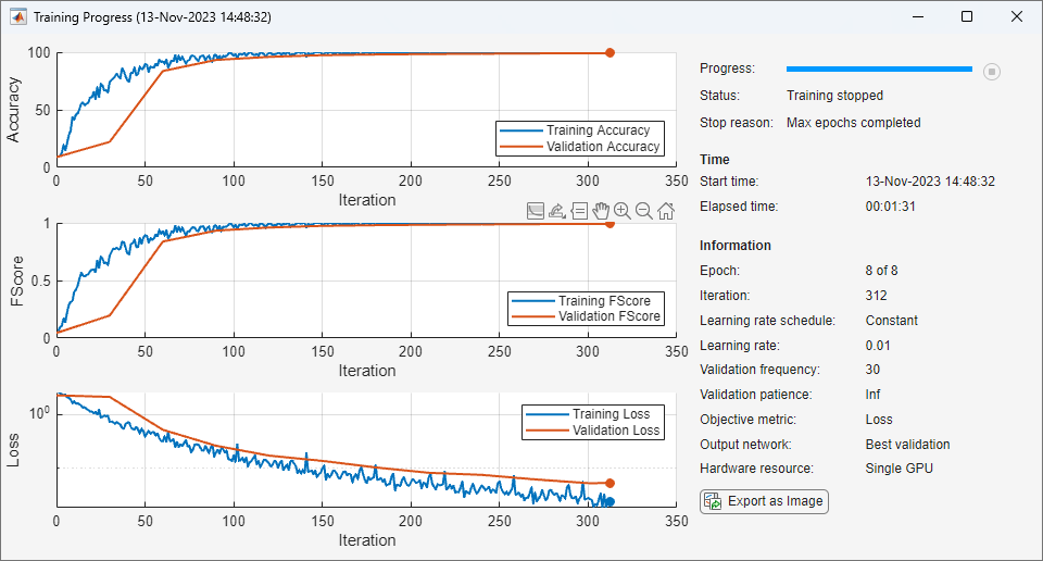
Specify options for network training. To validate the network at regular intervals during training, specify validation data. Record the metric values for the accuracy and F-score. To plot training progress during training, set the Plots training option to "training-progress".

options = trainingOptions("sgdm", ... MaxEpochs=8, ... Metrics = ["accuracy","fscore"], ... ValidationData={XTest,labelsTest}, ... ValidationFrequency=30, ... Verbose=false, ... Plots="training-progress");

Train the network.

net = trainnet(XTrain,labelsTrain,net,"crossentropy",options);

Stop Training Early Using Metrics

Use metrics for early stopping and to return the best network.

Load the training data, which contains 5000 images of digits. Set aside 1000 of the images for network validation.

[XTrain,YTrain] = digitTrain4DArrayData;

idx = randperm(size(XTrain,4),1000); XValidation = XTrain(:,:,:,idx); XTrain(:,:,:,idx) = []; YValidation = YTrain(idx); YTrain(idx) = [];

Construct a network to classify the digit image data.

net = dlnetwork;

layers = [ imageInputLayer([28 28 1]) convolution2dLayer(3,8,Padding="same") batchNormalizationLayer reluLayer
fullyConnectedLayer(10) softmaxLayer];

net = addLayers(net,layers);

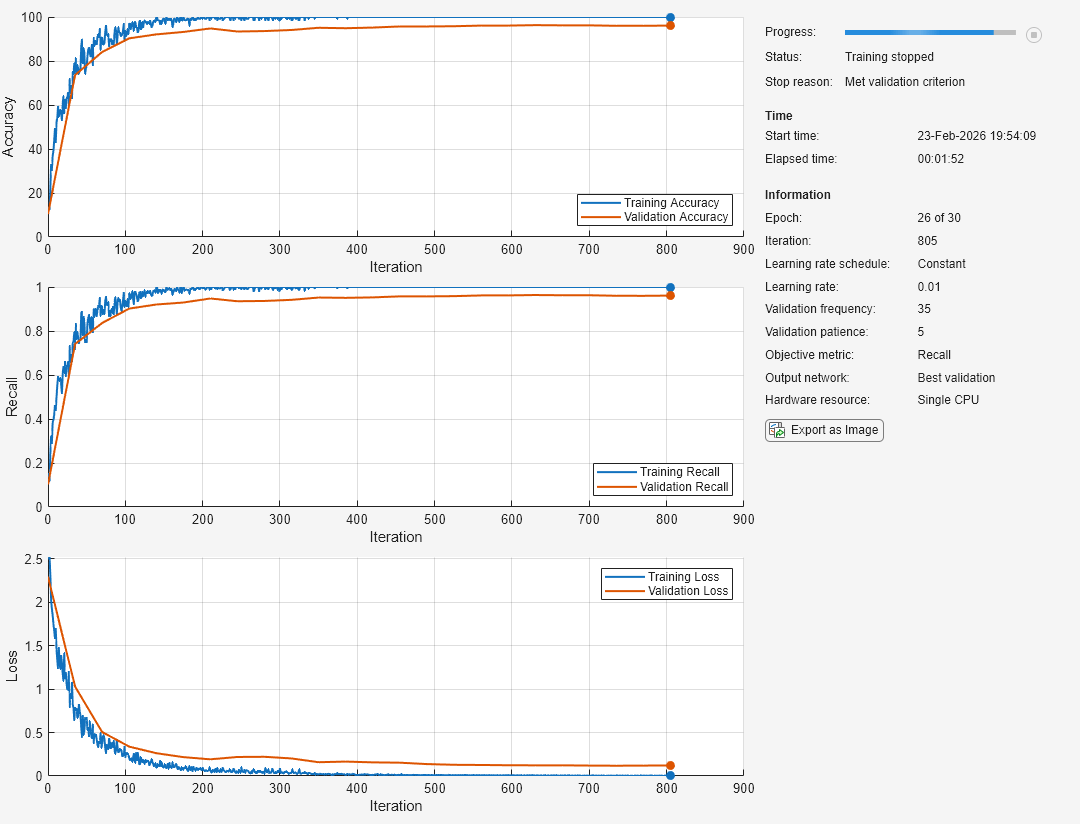
Specify the training options:

Use an SGDM solver for training.
Monitor training performance by specifying validation data and validation frequency.
Track the accuracy and recall during training. To return the network with the best recall value, specify "recall" as the objective metric and set the output network to "best-validation".
Specify the validation patience as 5 so training stops if the recall has not decreased for five iterations.
Visualize network training progress plot.
Suppress the verbose output.

options = trainingOptions("sgdm", ... ValidationData={XValidation,YValidation}, ... ValidationFrequency=35, ... ValidationPatience=5, ... Metrics=["accuracy","recall"], ... ObjectiveMetricName="recall", ... OutputNetwork="best-validation", ... Plots="training-progress", ... Verbose=false);

Train the network.

net = trainnet(XTrain,YTrain,net,"crossentropy",options);

Input Arguments

collapse all

`solverName` — Solver for training neural network

"sgdm" | "rmsprop" | "adam" | "lbfgs" (since R2023b) | "lm" (since R2024b)

Solver for training neural network, specified as one of these values:

"sgdm" — Stochastic gradient descent with momentum (SGDM). SGDM is a stochastic solver. For additional training options, see Stochastic Solver Options. For more information, see Stochastic Gradient Descent with Momentum.
"rmsprop" — Root mean square propagation (RMSProp). RMSProp is a stochastic solver. For additional training options, see Stochastic Solver Options. For more information, see Root Mean Square Propagation.
"adam" — Adaptive moment estimation (Adam). Adam is a stochastic solver. For additional training options, see Stochastic Solver Options. For more information, see Adaptive Moment Estimation.
"lbfgs" (since R2023b) — Limited-memory Broyden–Fletcher–Goldfarb–Shanno (L-BFGS). L-BFGS is a batch solver. Use the L-BFGS algorithm for small networks and data sets that you can process in a single batch. For additional training options, seeBatch Solver Options. For more information, see Limited-Memory BFGS.
"lm" (since R2024b) — Levenberg–Marquardt (LM). LM is a batch solver.Use the LM algorithm for regression networks with small numbers of learnable parameters, where you can process the data set in a single batch. If solverName is "lm", then the lossFcn argument of the trainnet function must be"mse" or"l2loss". For additional training options, see Batch Solver Options. For more information, see Levenberg–Marquardt.

The trainBERTDocumentClassifier (Text Analytics Toolbox) function supports the "sgdm", "rmsprop", and"adam" solvers only.

Name-Value Arguments

Specify optional pairs of arguments asName1=Value1,...,NameN=ValueN, where Name is the argument name and Value is the corresponding value. Name-value arguments must appear after other arguments, but the order of the pairs does not matter.

Before R2021a, use commas to separate each name and value, and enclose Name in quotes.

Example: Plots="training-progress",Metrics="accuracy",Verbose=false specifies to disable the verbose output and display the training progress in a plot that also includes the accuracy metric.

Monitoring

collapse all

`Plots` — Plots to display during neural network training

"none" (default) | "training-progress"

Plots to display during neural network training, specified as one of these values:

"none" — Do not display plots during training.
"training-progress" — Plot training progress.

The contents of the plot depends on the solver that you use.

When the solverName argument is"sgdm","adam", or"rmsprop", the plot shows the mini-batch loss, validation loss, training mini-batch and validation metrics specified by theMetrics option, and additional information about the training progress.
When the solverName argument is"lbfgs" or"lm", the plot shows the training and validation loss, training and validation metrics specified by the Metrics option, and additional information about the training progress.

To programmatically open and close the training progress plot after training, use the show and close functions with the second output of the trainnet function. You can use the show function to view the training progress even if the Plots training option is specified as "none".

To switch the y-axis scale to logarithmic, use the axes toolbar. Training plot axes toolbar with log scale enabled and the tooltip "Log scale y-axis".

For more information about the plot, see Monitor Deep Learning Training Progress.

`Metrics` — Metrics to monitor

Since R2023b

Metrics to monitor, specified as one of these values:

Built-in metric or loss function name — Specify metrics as a string scalar, character vector, or a cell array or string array of one or more of these names:
- Metrics:
  * "accuracy" — Accuracy (also known as top-1 accuracy)
  * "auc" — Area under ROC curve (AUC)
  * "fscore" — F-score (also known as F1-score)
  * "precision" — Precision
  * "recall" — Recall
  * "rmse" — Root mean squared error
  * "mape" — Mean absolute percentage error (MAPE) (since R2024b)
- Loss functions:
  * "crossentropy" — Cross-entropy loss for classification tasks. (since R2024b)
  * "indexcrossentropy" — Index cross-entropy loss for classification tasks. (since R2024b)
  * "binary-crossentropy" — Binary cross-entropy loss for binary and multilabel classification tasks. (since R2024b)
  * "mae" /"mean-absolute-error" / "l1loss" — Mean absolute error for regression tasks. (since R2024b)
  * "mse" /"mean-squared-error" / "l2loss" — Mean squared error for regression tasks. (since R2024b)
  * "huber" — Huber loss for regression tasks (since R2024b)

Note that setting the loss function as "crossentropy" and specifying "index-crossentropy" as a metric or setting the loss function as "index-crossentropy" and specifying"crossentropy" as a metric is not supported.

Built-in metric object — If you need more flexibility, you can use built-in metric objects. The software supports these built-in metric objects:
- AccuracyMetric
- AUCMetric
- FScoreMetric
- PrecisionMetric
- RecallMetric
- RMSEMetric
- MAPEMetric (since R2024b)
  When you create a built-in metric object, you can specify additional options such as the averaging type and whether the task is single-label or multilabel.
Custom metric function handle — If the metric you need is not a built-in metric, then you can specify custom metrics using a function handle. The function must have the syntax metric = metricFunction(Y,T), where Y corresponds to the network predictions and T corresponds to the target responses. For networks with multiple outputs, the syntax must be metric = metricFunction(Y1,…,YN,T1,…TM), where N is the number of outputs and M is the number of targets. For more information, seeDefine Custom Metric Function.
Note
When you have data in mini-batches, the software computes the metric for each mini-batch and then returns the average of those values. For some metrics, this behavior can result in a different metric value than if you compute the metric using the whole data set at once. In most cases, the values are similar. To use a custom metric that is not batch-averaged for the data, you must create a custom metric object. For more information, see Define Custom Deep Learning Metric Object.
deep.DifferentiableFunction object (since R2024a) — Function object with custom backward function. For categorical targets, the software automatically converts the categorical values to one-hot encoded vectors and passes them to the metric function. For more information, see Define Custom Deep Learning Operations.
Custom metric object — If you need greater customization, then you can define your own custom metric object. For an example that shows how to create a custom metric, seeDefine Custom Metric Object. For general information about creating custom metrics, see Define Custom Deep Learning Metric Object.

If you specify a metric as a function handle, a deep.DifferentiableFunction object, or a custom metric object and train the neural network using thetrainnet function, then the layout of the targets that the software passes to the metric depends on the data type of the targets, and the loss function that you specify in the trainnet function and the other metrics that you specify:

If the targets are numeric arrays, then the software passes the targets to the metric directly.
If the loss function is "index-crossentropy" and the targets are categorical arrays, then the software automatically converts the targets to numeric class indices and passes them to the metric.
For other loss functions, if the targets are categorical arrays, then the software automatically converts the targets to one-hot encoded vectors and then passes them to the metric.

This option supports the trainnet andtrainBERTDocumentClassifier (Text Analytics Toolbox) functions only.

Example: Metrics=["accuracy","fscore"]

Example: Metrics={"accuracy",@myFunction,precisionObj}

`ObjectiveMetricName` — Name of objective metric

"loss" (default) | string scalar | character vector

Since R2024a

Name of objective metric to use for early stopping and returning the best network, specified as a string scalar or character vector.

The metric name must be "loss" or match the name of a metric specified by the Metrics argument. Metrics specified using function handles are not supported. To specify the ObjectiveMetricName value as the name of a custom metric, the value of the Maximize property of the custom metric object must be nonempty. For more information, see Define Custom Deep Learning Metric Object.

For more information about specifying the objective metric for early stopping, see ValidationPatience. For more information about returning the best network using the objective metric, see OutputNetwork.

Data Types: char | string

`Verbose` — Flag to display training progress information

1 (true) (default) | 0 (false)

Flag to display training progress information in the command window, specified as 1 (true) or 0 (false).

The content of the verbose output depends on the type of solver.

For stochastic solvers (SGDM, Adam, and RMSProp), the table contains these variables:

Variable	Description
Iteration	Iteration number.
Epoch	Epoch number.
TimeElapsed	Time elapsed in hours, minutes, and seconds.
LearnRate	Learning rate.
TrainingLoss	Training loss.
ValidationLoss	Validation loss. If you do not specify validation data, then the software does not display this information.

For batch solvers (L-BFGS and LM), the table contains these variables:

Variable	Description
Iteration	Iteration number.
TimeElapsed	Time elapsed in hours, minutes, and seconds.
TrainingLoss	Training loss.
ValidationLoss	Validation loss. If you do not specify validation data, then the software does not display this information.
GradientNorm	Norm of the gradients.
StepNorm	Norm of the steps.

If you specify additional metrics in the training options, then they also appear in the verbose output. For example, if you set the Metrics training option to "accuracy", then the information includes theTrainingAccuracy and ValidationAccuracy variables.

When training stops, the verbose output displays the reason for stopping.

To specify validation data, use the ValidationData training option.

`VerboseFrequency` — Frequency of verbose printing

50 (default) | positive integer

Frequency of verbose printing, which is the number of iterations between printing to the Command Window, specified as a positive integer.

If you validate the neural network during training, then the software also prints to the command window every time validation occurs.

To enable this property, set the Verbose training option to1 (true).

`OutputFcn` — Output functions

function handle | cell array of function handles

Output functions to call during training, specified as a function handle or cell array of function handles. The software calls the functions once before the start of training, after each iteration, and once when training is complete.

The functions must have the syntax stopFlag = f(info), where info is a structure containing information about the training progress, and stopFlag is a scalar that indicates to stop training early. If stopFlag is 1 (true), then the software stops training. Otherwise, the software continues training.

The trainnet function passes the output function the structure info.

For stochastic solvers (SGDM, Adam, and RMSProp),info contains these fields:

Field	Description
Epoch	Epoch number
Iteration	Iteration number
TimeElapsed	Time since start of training
LearnRate	Iteration learn rate
TrainingLoss	Iteration training loss
ValidationLoss	Validation loss, if specified and evaluated at iteration.
State	Iteration training state, specified as "start", "iteration", or "done".

For batch solvers (L-BFGS and LM), info contains these fields:

Field	Description
Iteration	Iteration number
TimeElapsed	Time elapsed in hours, minutes, and seconds
TrainingLoss	Training loss
ValidationLoss	Validation loss. If you do not specify validation data, then the software does not display this information.
GradientNorm	Norm of the gradients
StepNorm	Norm of the steps
State	Iteration training state, specified as "start", "iteration", or "done".

If you specify additional metrics in the training options, then they also appear in the training information. For example, if you set theMetrics training option to "accuracy", then the information includes the TrainingAccuracy andValidationAccuracy fields.

If a field is not calculated or relevant for a certain call to the output functions, then that field contains an empty array.

For an example showing how to use output functions, seeCustom Stopping Criteria for Deep Learning Training.

Data Types: function_handle | cell

Data Formats

collapse all

`InputDataFormats` — Description of input data dimensions

"auto" (default) | string array | cell array of character vectors | character vector

Since R2023b

Description of the input data dimensions, specified as a string array, character vector, or cell array of character vectors.

If InputDataFormats is "auto", then the software uses the formats expected by the network input. Otherwise, the software uses the specified formats for the corresponding network input.

A data format is a string of characters, where each character describes the type of the corresponding data dimension.

The characters are:

"S" — Spatial
"C" — Channel
"B" — Batch
"T" — Time
"U" — Unspecified

For example, consider an array containing a batch of sequences where the first, second, and third dimensions correspond to channels, observations, and time steps, respectively. You can specify that this array has the format "CBT" (channel, batch, time).

You can specify multiple dimensions labeled "S" or "U". You can use the labels "C", "B", and"T" once each, at most. The software ignores singleton trailing"U" dimensions after the second dimension.

For a neural networks with multiple inputs net, specify an array of input data formats, where InputDataFormats(i) corresponds to the input net.InputNames(i).

For more information, see Deep Learning Data Formats.

Data Types: char | string | cell

`TargetDataFormats` — Description of target data dimensions

"auto" (default) | string array | cell array of character vectors | character vector

Since R2023b

Description of the target data dimensions, specified as one of these values:

"auto" — If the target data has the same number of dimensions as the input data, then the trainnet function uses the format specified by InputDataFormats. If the target data has a different number of dimensions to the input data, then the trainnet function uses the format expected by the loss function.
String array, character vector, or cell array of character vectors — The trainnet function uses the data formats you specify.

A data format is a string of characters, where each character describes the type of the corresponding data dimension.

The characters are:

"S" — Spatial
"C" — Channel
"B" — Batch
"T" — Time
"U" — Unspecified

For more information, see Deep Learning Data Formats.

Data Types: char | string | cell

Stochastic Solver Options

collapse all

`MaxEpochs` — Maximum number of epochs

30 (default) | positive integer

Maximum number of epochs (full passes of the data) to use for training, specified as a positive integer.

This option supports stochastic solvers only (when the solverName argument is "sgdm", "adam", or"rmsprop").

`MiniBatchSize` — Size of mini-batch

128 (default) | positive integer

Size of the mini-batch to use for each training iteration, specified as a positive integer. A mini-batch is a subset of the training set that is used to evaluate the gradient of the loss function and update the weights.

If the mini-batch size does not evenly divide the number of training samples, then the software discards the training data that does not fit into the final complete mini-batch of each epoch. If the mini-batch size is smaller than the number of training samples, then the software does not discard any data.

This option supports stochastic solvers only (when the solverName argument is "sgdm", "adam", or"rmsprop").

Tip

For best performance, if you are training a network using a datastore with aReadSize property, such as an imageDatastore, then set the ReadSize property andMiniBatchSize training option to the same value. If you are training a network using a datastore with a MiniBatchSize property, such as an augmentedImageDatastore, then set the MiniBatchSize property of the datastore and the MiniBatchSize training option to the same value.

`Shuffle` — Option for data shuffling

"once" (default) | "never" | "every-epoch"

Option for data shuffling, specified as one of these values:

"once" — Shuffle the training and validation data once before training.
"never" — Do not shuffle the data.
"every-epoch" — Shuffle the training data before each training epoch, and shuffle the validation data before each neural network validation. If the mini-batch size does not evenly divide the number of training samples, then the software discards the training data that does not fit into the final complete mini-batch of each epoch. To avoid discarding the same data every epoch, set the Shuffle training option to "every-epoch".

This option supports stochastic solvers only (when the solverName argument is "sgdm", "adam", or"rmsprop").

`InitialLearnRate` — Initial learning rate

positive scalar

Initial learning rate used for training, specified as a positive scalar.

If the learning rate is too low, then training can take a long time. If the learning rate is too high, then training might reach a suboptimal result or diverge.

This option supports stochastic solvers only (when the solverName argument is "sgdm", "adam", or"rmsprop").

When solverName is"sgdm", the default value is0.01. WhensolverName is"rmsprop" or"adam", the default value is0.001.

`LearnRateSchedule` — Learning rate schedule

Learning rate schedule, specified as a character vector or string scalar of a built-in learning rate schedule name, a string array of names, a built-in or custom learning rate schedule object, a function handle, or a cell array of names, metric objects, and function handles.

This option supports stochastic solvers only (when the solverName argument is "sgdm", "adam", or"rmsprop").

Built-In Learning Rate Schedule Names

Specify learning rate schedules as a string scalar, character vector, or a string or cell array of one or more of these names:

Name	Description	Plot
"none"	No learning rate schedule. This schedule keeps the learning rate constant.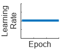
"piecewise"	Piecewise learning rate schedule. Every 10 epochs, this schedule drops the learn rate by a factor of 10.
"warmup" (since R2024b)	Warm-up learning rate schedule. For 5 iterations, this schedule ramps up the learning rate to the base learning rate.
"polynomial" (since R2024b)	Polynomial learning rate schedule. Every epoch, this schedule drops the learning rate using a power law with a unitary exponent.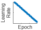
"exponential" (since R2024b)	Exponential learning rate schedule. Every epoch, this schedule decays the learning rate by a factor of 10.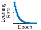
"cosine" (since R2024b)	Cosine learning rate schedule. Every epoch, this schedule drops the learn rate using a cosine formula.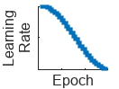
"cyclical" (since R2024b)	Cyclical learning rate schedule. For periods of 10 epochs, this schedule increases the learning rate from the base learning rate for 5 epochs and then decreases the learning rate for 5 epochs.

Built-In Learning Rate Schedule Object (since R2024b)

If you need more flexibility than what the string options provide, you can use built-in learning rate schedule objects:

piecewiseLearnRate — A piecewise learning rate schedule object drops the learning rate periodically by multiplying it by a specified factor. Use this object to customize the drop factor and period of the piecewise schedule.
Before R2024b: Customize the piecewise drop factor and period using the LearnRateDropFactor andLearnRateDropPeriod training options, respectively.
warmupLearnRate — A warm-up learning rate schedule object ramps up the learning for a specified number of iterations. Use this object to customize the initial and final learning rate factors and the number of steps of the warm up schedule.
polynomialLearnRate — A polynomial learning rate schedule drops the learning rate using a power law. Use this object to customize the initial and final learning rate factors, the exponent, and the number of steps of the polynomial schedule.
exponentialLearnRate — An exponential learning rate schedule decays the learning rate by a specified factor. Use this object to customize the drop factor and period of the exponential schedule.
cosineLearnRate — A cosine learning rate schedule object drops the learning rate using a cosine curve and incorporates warm restarts. Use this object to customize the initial and final learning rate factors, the period, and the period growth factor of the cosine schedule.
cyclicalLearnRate — A cyclical learning rate schedule periodically increases and decreases the learning rate. Use this option to customize the maximum factor, period, and step ratio of the cyclical schedule.

Custom Learning Rate Schedule (since R2024b)

For additional flexibility, you can define a custom learning rate schedule as a function handle or custom class that inherits from deep.LearnRateSchedule.

Custom learning rate schedule function handle — If the learning rate schedule you need is not a built-in learning rate schedule, then you can specify custom learning rate schedules using a function handle. To specify a custom schedule, use a function handle with the syntax learningRate = f(baseLearningRate,epoch), wherebaseLearningRate is the base learning rate, andepoch is the epoch number.
Custom learn rate schedule object — If you need more flexibility that what function handles provide, then you can define a custom learning rate schedule class that inherits from deep.LearnRateSchedule.

Multiple Learning Rate Schedules (since R2024b)

You can combine multiple learning rate schedules by specifying multiple schedules as a string or cell array and then the software applies the schedules in order, starting with the first element. At most one of the schedules can be infinite (schedules than continue indefinitely, such as "cyclical" and objects with the NumSteps property set to Inf) and the infinite schedule must be the last element of the array.

`Momentum` — Contribution of previous step

0.9 (default) | scalar from 0 to1

Contribution of the parameter update step of the previous iteration to the current iteration of stochastic gradient descent with momentum, specified as a scalar from 0 to 1.

A value of 0 means no contribution from the previous step, whereas a value of 1 means maximal contribution from the previous step. The default value works well for most tasks.

This option supports the SGDM solver only (when the solverName argument is"sgdm").

For more information, see Stochastic Gradient Descent with Momentum.

`GradientDecayFactor` — Decay rate of gradient moving average

0.9 (default) | nonnegative scalar less than 1

Decay rate of gradient moving average for the Adam solver, specified as a nonnegative scalar less than 1. The gradient decay rate is denoted by β1 in the Adaptive Moment Estimation section.

This option supports the Adam solver only (when the solverName argument is"adam").

For more information, see Adaptive Moment Estimation.

`SquaredGradientDecayFactor` — Decay rate of squared gradient moving average

nonnegative scalar less than 1

Decay rate of squared gradient moving average for the Adam and RMSProp solvers, specified as a nonnegative scalar less than 1. The squared gradient decay rate is denoted byβ2 in[4].

Typical values of the decay rate are 0.9, 0.99, and 0.999, corresponding to averaging lengths of 10, 100, and 1000 parameter updates, respectively.

This option supports the Adam and RMSProp solvers only (when the solverName argument is "adam" or"rmsprop").

The default value is 0.999 for the Adam solver. The default value is 0.9 for the RMSProp solver.

For more information, see Adaptive Moment Estimation and Root Mean Square Propagation.

`Epsilon` — Denominator offset

1e-8 (default) | positive scalar

Denominator offset for Adam and RMSProp solvers, specified as a positive scalar.

The solver adds the offset to the denominator in the neural network parameter updates to avoid division by zero. The default value works well for most tasks.

This option supports the Adam and RMSProp solvers only (when the solverName argument is "adam" or"rmsprop").

For more information, see Adaptive Moment Estimation and Root Mean Square Propagation.

`LearnRateDropFactor` — Factor for dropping the learning rate

0.1 (default) | scalar from 0 to1

Factor for dropping the learning rate, specified as a scalar from 0 to 1. This option is valid only when the LearnRateSchedule training option is "piecewise".

LearnRateDropFactor is a multiplicative factor to apply to the learning rate every time a certain number of epochs passes. Specify the number of epochs using the LearnRateDropPeriod training option.

This option supports stochastic solvers only (when the solverName argument is "sgdm", "adam", or"rmsprop").

Tip

To customize the piecewise learning rate schedule, use a piecewiseLearnRate object. A piecewiseLearnRate object is recommended over the LearnRateDropFactor and LearnRateDropPeriod training options because it provides additional control over the drop frequency. (since R2024b)

`LearnRateDropPeriod` — Number of epochs for dropping the learning rate

10 (default) | positive integer

Number of epochs for dropping the learning rate, specified as a positive integer. This option is valid only when the LearnRateSchedule training option is "piecewise".

The software multiplies the global learning rate with the drop factor every time the specified number of epochs passes. Specify the drop factor using the LearnRateDropFactor training option.

This option supports stochastic solvers only (when the solverName argument is "sgdm", "adam", or"rmsprop").

Tip

Batch Solver Options

collapse all

`MaxIterations` — Maximum number of iterations

1000 (default) | positive integer

Since R2023b

Maximum number of iterations to use for training, specified as a positive integer.

The L-BFGS solver is a full-batch solver, which means that it processes the entire training set in a single iteration.

This option supports batch solvers only (when the solverName argument is "lbfgs" or "lm").

`GradientTolerance` — Relative gradient tolerance

1e-5 (default) | positive scalar

Since R2023b

Relative gradient tolerance, specified as a positive scalar.

The software stops training when the relative gradient is less than or equal to GradientTolerance.

This option supports batch solvers only (when the solverName argument is "lbfgs" or "lm").

`StepTolerance` — Step size tolerance

1e-5 (default) | positive scalar

Since R2023b

Step size tolerance, specified as a positive scalar.

The software stops training when the step that the algorithm takes is less than or equal toStepTolerance.

This option supports batch solvers only (when the solverName argument is "lbfgs" or "lm").

`LineSearchMethod` — Method to find suitable learning rate

"weak-wolfe" (default) | "strong-wolfe" | "backtracking"

Since R2023b

Method to find suitable learning rate, specified as one of these values:

"weak-wolfe" — Search for a learning rate that satisfies the weak Wolfe conditions. This method maintains a positive definite approximation of the inverse Hessian matrix.
"strong-wolfe" — Search for a learning rate that satisfies the strong Wolfe conditions. This method maintains a positive definite approximation of the inverse Hessian matrix.
"backtracking" — Search for a learning rate that satisfies sufficient decrease conditions. This method does not maintain a positive definite approximation of the inverse Hessian matrix.

This option supports the L-BFGS solver only (when the solverName argument is"lbfgs").

`HistorySize` — Number of state updates to store

10 (default) | positive integer

Since R2023b

Number of state updates to store, specified as a positive integer. Values between 3 and 20 suit most tasks.

The L-BFGS algorithm uses a history of gradient calculations to approximate the Hessian matrix recursively. For more information, see Limited-Memory BFGS.

This option supports the L-BFGS solver only (when the solverName argument is"lbfgs").

`InitialInverseHessianFactor` — Initial value that characterizes approximate inverse Hessian matrix

1 (default) | positive scalar

Since R2023b

Initial value that characterizes the approximate inverse Hessian matrix, specified as a positive scalar.

To save memory, the L-BFGS algorithm does not store and invert the dense Hessian matrix_B_. Instead, the algorithm uses the approximation Bk−m−1≈λkI, where m is the history size, the inverse Hessian factor λk is a scalar, and I is the identity matrix. The algorithm then stores the scalar inverse Hessian factor only. The algorithm updates the inverse Hessian factor at each step.

The initial inverse hessian factor is the value of λ0.

For more information, see Limited-Memory BFGS.

This option supports the L-BFGS solver only (when the solverName argument is"lbfgs").

`MaxNumLineSearchIterations` — Maximum number of line search iterations

20 (default) | positive integer

Since R2023b

Maximum number of line search iterations to determine the learning rate, specified as a positive integer.

This option supports the L-BFGS solver only (when the solverName argument is"lbfgs").

`InitialStepSize` — Approximate maximum absolute value of the first optimization step

[] (default) | "auto" | real finite scalar

Since R2024b

Initial step size, specified as one of these values:

[] — Do not use an initial step size to determine the initial Hessian approximation.
"auto" — Determine the initial step size automatically. The software uses an initial step size of ‖s0‖∞=12‖W0‖∞+0.1, where W0 are the initial learnable parameters of the network.
Positive real scalar — Use the specified value as the initial step size ‖s0‖∞.

If InitialStepSize is "auto" or a positive real scalar, then the software approximates the initial inverse Hessian using λ0=‖s0‖∞‖∇J(W0)‖∞, where λ0 is the initial inverse Hessian factor and ∇J(W0) denotes the gradients of the loss with respect to the initial learnable parameters. For more information, see Limited-Memory BFGS.

This option supports the L-BFGS solver only (when the solverName argument is"lbfgs").

`InitialDampingFactor` — Initial damping factor

0.001 (default) | positive scalar

Since R2024b

Initial damping factor, specified as a positive scalar.

This option supports the LM solver only (when the solverName argument is "lm").

`MaxDampingFactor` — Maximum damping factor

1e10 (default) | positive scalar

Since R2024b

Maximum damping factor, specified as a positive scalar.

This option supports the LM solver only (when the solverName argument is "lm").

`DampingIncreaseFactor` — Factor for increasing damping factor

10 (default) | positive scalar greater than 1

Since R2024b

Factor for increasing damping factor, specified as a positive scalar greater than 1.

This option supports the LM solver only (when the solverName argument is "lm").

`DampingDecreaseFactor` — Factor for decreasing damping factor

0.1 (default) | positive scalar less than 1

Since R2024b

Factor for decreasing damping factor, specified as a positive scalar less than 1.

Validation

collapse all

`ValidationData` — Data to use for validation during training

[] (default) | datastore | table | cell array | minibatchqueue object (since R2024a)

Data to use for validation during training, specified as [], a datastore, a table, a cell array, or a minibatchqueue object that contains the validation predictors and targets.

During training, the software uses the validation data to calculate the validation loss and metric values. To specify the validation frequency, use the ValidationFrequency training option. You can also use the validation data to stop training automatically when the validation objective metric stops improving. By default, the objective metric is set to the loss. To turn on automatic validation stopping, use the ValidationPatience training option.

If ValidationData is [], then the software does not validate the neural network during training.

If your neural network has layers that behave differently during prediction than during training (for example, dropout layers), then the validation loss can be lower than the training loss.

The software shuffles the validation data according to the Shuffle training option. IfShuffle is "every-epoch", then the software shuffles the validation data before each neural network validation.

The supported formats depend on the training function that you use.

`trainnet` Function

Specify the validation data as a datastore, minibatchqueue object, or the cell array {predictors,targets}, where predictors contains the validation predictors and targets contains the validation targets. Specify the validation predictors and targets using any of the formats supported by the trainnet function.

For more information, see the input arguments of the trainnet function.

`trainBERTDocumentClassifier` Function (Text Analytics Toolbox)

Specify the validation data as one of these values:

Cell array {documents,targets}, wheredocuments contains the input documents, andtargets contains the document labels.
Table, where the first variable contains the input documents and the second variable contains the document labels.

For more information, see the input arguments of the trainBERTDocumentClassifier (Text Analytics Toolbox) function.

`ValidationFrequency` — Frequency of neural network validation

50 (default) | positive integer

Frequency of neural network validation in number of iterations, specified as a positive integer.

The ValidationFrequency value is the number of iterations between evaluations of validation metrics. To specify validation data, use the ValidationData training option.

`ValidationPatience` — Patience of validation stopping

Inf (default) | positive integer

Patience of validation stopping of neural network training, specified as a positive integer or Inf.

ValidationPatience specifies the number of times that the objective metric on the validation set can be worse than or equal to the previous best value before neural network training stops. If ValidationPatience is Inf, then the values of the validation metric do not cause training to stop early. The software aims to maximize or minimize the metric, as specified by the Maximize property of the metric. When the objective metric is "loss", the software aims to minimize the loss value.

The returned neural network depends on the OutputNetwork training option. To return the neural network with the best validation metric value, set the OutputNetwork training option to "best-validation".

Before R2024a: The software computes the validation patience using the validation loss value.

`OutputNetwork` — Neural network to return when training completes

"auto" (default) | "last-iteration" | "best-validation"

Neural network to return when training completes, specified as one of the following:

"auto" – Use "best-validation" ifValidationData is specified. Otherwise, use"last-iteration".
"best-validation" – Return the neural network corresponding to the training iteration with the best validation metric value, where the metric to optimize is specified by theObjectiveMetricName option. To use this option, you must specify the ValidationData training option.
"last-iteration" – Return the neural network corresponding to the last training iteration.

Regularization and Normalization

collapse all

`L2Regularization` — Factor for L2 regularization

0.0001 (default) | nonnegative scalar

Factor for L2 regularization (weight decay), specified as a nonnegative scalar. For more information, see L2 Regularization.

This option does not support the LM solver (when the solverName argument is "lm").

`ResetInputNormalization` — Option to reset input layer normalization

1 (true) (default) | 0 (false)

Option to reset input layer normalization, specified as one of the following:

1 (true) — Reset the input layer normalization statistics and recalculate them at training time.
0 (false) — Calculate normalization statistics at training time when they are empty.

`BatchNormalizationStatistics` — Mode to evaluate statistics in batch normalization layers

"auto" (default) | "population" | "moving"

Mode to evaluate the statistics in batch normalization layers, specified as one of the following:

"population" — Use the population statistics. After training, the software finalizes the statistics by passing through the training data once more and uses the resulting mean and variance.
"moving" — Approximate the statistics during training using a running estimate given by update steps
where μ* and σ2* denote the updated mean and variance, respectively, λμ and λσ2 denote the mean and variance decay values, respectively, μ^ and σ2^ denote the mean and variance of the layer input, respectively, and μ and σ2 denote the latest values of the moving mean and variance values, respectively. After training, the software uses the most recent value of the moving mean and variance statistics. This option supports CPU and single GPU training only.
"auto" — Use the "moving" option.

Gradient Clipping

collapse all

`GradientThreshold` — Gradient threshold

Inf (default) | positive scalar

Gradient threshold, specified as Inf or a positive scalar. If the gradient exceeds the value of GradientThreshold, then the gradient is clipped according to the GradientThresholdMethod training option.

For more information, see Gradient Clipping.

This option does not support the LM solver (when the solverName argument is "lm").

`GradientThresholdMethod` — Gradient threshold method

"l2norm" (default) | "global-l2norm" | "absolute-value"

Gradient threshold method used to clip gradient values that exceed the gradient threshold, specified as one of the following:

"l2norm" — If the L2 norm of the gradient of a learnable parameter is larger than GradientThreshold, then scale the gradient so that the L2 norm equals GradientThreshold.
"global-l2norm" — If the global L2 norm, L, is larger than GradientThreshold, then scale all gradients by a factor of GradientThreshold/L. The global L2 norm considers all learnable parameters.
"absolute-value" — If the absolute value of an individual partial derivative in the gradient of a learnable parameter is larger than GradientThreshold, then scale the partial derivative to have magnitude equal to GradientThreshold and retain the sign of the partial derivative.

For more information, see Gradient Clipping.

This option does not support the LM solver (when the solverName argument is "lm").

Sequence

collapse all

`SequenceLength` — Option to pad or truncate sequences

"longest" (default) | "shortest"

Option to pad, truncate, or split input sequences, specified as one of these values:

"longest" — Pad sequences in each mini-batch to have the same length as the longest sequence. This option does not discard any data, though padding can introduce noise to the neural network.
"shortest" — Truncate sequences in each mini-batch to have the same length as the shortest sequence. This option ensures that no padding is added, at the cost of discarding data.

To learn more about the effect of padding and truncating sequences, see Sequence Padding and Truncation.

`SequencePaddingDirection` — Direction of padding or truncation

"right" (default) | "left"

Direction of padding or truncation, specified as one of these options:

"right" — Pad or truncate sequences on the right. The sequences start at the same time step and the software truncates or adds padding to the end of each sequence.
"left" — Pad or truncate sequences on the left. The software truncates or adds padding to the start of each sequence so that the sequences end at the same time step.

Because recurrent layers process sequence data one time step at a time, when the recurrent layer OutputMode property is "last", any padding in the final time steps can negatively influence the layer output. To pad or truncate sequence data on the left, set the SequencePaddingDirection argument to "left".

For sequence-to-sequence neural networks (when the OutputMode property is"sequence" for each recurrent layer), any padding in the first time steps can negatively influence the predictions for the earlier time steps. To pad or truncate sequence data on the right, set the SequencePaddingDirection option to "right".

To learn more about the effects of padding and truncating sequences, see Sequence Padding and Truncation.

`SequencePaddingValue` — Value by which to pad input sequences

0 (default) | scalar

Value by which to pad the input sequences, specified as a scalar.

Do not pad sequences with NaN, because doing so can propagate errors through the neural network.

Hardware and Acceleration

collapse all

`ExecutionEnvironment` — Hardware resource for training neural network

Hardware resource for training neural network, specified as one of these values:

"auto" – Use a local GPU if one is available. Otherwise, use the local CPU.
"cpu" – Use the local CPU.
"gpu" – Use the local GPU.
"multi-gpu" – Use multiple GPUs on one machine, using a local parallel pool based on your default cluster profile. If there is no current parallel pool, the software starts a parallel pool with pool size equal to the number of available GPUs.
"parallel-auto" – Use a local or remote parallel pool. If there is no current parallel pool, the software starts one using the default cluster profile. If the pool has access to GPUs, then only workers with a unique GPU perform training computation and excess workers become idle. If the pool does not have GPUs, then training takes place on all available CPU workers instead. (since R2024a)
Before R2024a: Use "parallel" instead.
"parallel-cpu" – Use CPU resources in a local or remote parallel pool, ignoring any GPUs. If there is no current parallel pool, the software starts one using the default cluster profile. (since R2023b)
"parallel-gpu" – Use GPUs in a local or remote parallel pool. Excess workers become idle. If there is no current parallel pool, the software starts one using the default cluster profile. (since R2023b)

The "gpu", "multi-gpu","parallel-auto", "parallel-cpu", and"parallel-gpu" options require Parallel Computing Toolbox™. To use a GPU for deep learning, you must also have a supported GPU device. For information on supported devices, see GPU Computing Requirements (Parallel Computing Toolbox). If you choose one of these options and Parallel Computing Toolbox or a suitable GPU is not available, then the software returns an error.

For more information on when to use the different execution environments, see Scale Up Deep Learning in Parallel, on GPUs, and in the Cloud.

To see an improvement in performance when training in parallel, try scaling up the MiniBatchSize and InitialLearnRate training options by the number of GPUs.

The "multi-gpu","parallel-auto","parallel-cpu", and"parallel-gpu" options support stochastic solvers only (when the solverName argument is"sgdm","adam", or"rmsprop").

`PreprocessingEnvironment` — Environment for fetching and preprocessing data

"serial" (default) | "background" | "parallel"

Since R2024a

Environment for fetching and preprocessing data from a datastore during training, specified as one of these values:

"serial" – Fetch and preprocess data in serial.
"background" – Fetch and preprocess data using the background pool.
"parallel" – Fetch and preprocess data using parallel workers. The software opens a parallel pool using the default profile, if a local pool is not currently open. Non-local parallel pools are not supported. Using this option requires Parallel Computing Toolbox. This option is not supported when training in parallel (when theExecutionEnvironment option is"parallel-auto", "parallel-cpu","parallel-gpu", or "multi-gpu").

To use the "background" or "parallel" options, the input datastore must be subsettable or partitionable. Custom datastores must implement the matlab.io.datastore.Subsettable class.

The "background" and "parallel" options are not supported when the Shuffle option is "never".

If you use the "background" and "parallel" options, then training is non-deterministic even if you use the deep.gpu.deterministicAlgorithms function.

Use the "background" option when your mini-batches require significant preprocessing. If your preprocessing is not supported on threads, or if you need to control the number of workers, use the "parallel" option. For more information about the preprocessing environment, see Preprocess Data in the Background or in Parallel.

This option supports stochastic solvers only (when the solverName argument is "sgdm", "adam", or"rmsprop").

Before R2024a: To preprocess data in parallel, set theDispatchInBackground training option to 1 (true).

`Acceleration` — Performance optimization

"auto" (default) | "none"

Since R2024a

Performance optimization, specified as one of these values:

"auto" – Automatically apply a number of optimizations suitable for the input network and hardware resources.
"none" – Disable all optimizations.

Checkpoints

collapse all

`CheckpointPath` — Path for saving checkpoint neural networks

"" (default) | string scalar | character vector

Path for saving the checkpoint neural networks, specified as a string scalar or character vector.

If you do not specify a path (that is, you use the default""), then the software does not save any checkpoint neural networks.
If you specify a path, then the software saves checkpoint neural networks to this path and assigns a unique name to each neural network. You can then load any checkpoint neural network and resume training from that neural network.
If the folder does not exist, then you must first create it before specifying the path for saving the checkpoint neural networks. If the path you specify does not exist, then the software throws an error.

Data Types: char | string

`CheckpointFrequency` — Frequency of saving checkpoint neural networks

positive integer

Frequency of saving checkpoint neural networks, specified as a positive integer.

If solverName is "lbfgs" or CheckpointFrequencyUnit is"iteration", then the software saves checkpoint neural networks everyCheckpointFrequency iterations. Otherwise, the software saves checkpoint neural networks every CheckpointFrequency epochs.

When solverName is"sgdm","adam", or"rmsprop", the default value is1. WhensolverName is"lbfgs" or"lm", the default value is30.

This option only has an effect whenCheckpointPath is nonempty.

`CheckpointFrequencyUnit` — Checkpoint frequency unit

"epoch" (default) | "iteration"

Checkpoint frequency unit, specified as "epoch" or "iteration".

If CheckpointFrequencyUnit is "epoch", then the software saves checkpoint neural networks every CheckpointFrequency epochs.

If CheckpointFrequencyUnit is "iteration", then the software saves checkpoint neural networks everyCheckpointFrequency iterations.

This option only has an effect when CheckpointPath is nonempty.

This option supports stochastic solvers only (when the solverName argument is "sgdm", "adam", or"rmsprop").

Output Arguments

Tips

For most deep learning tasks, you can use a pretrained neural network and adapt it to your own data. For an example showing how to use transfer learning to retrain a convolutional neural network to classify a new set of images, see Retrain Neural Network to Classify New Images. Alternatively, you can create and train neural networks from scratch using the trainnet andtrainingOptions functions.
If the trainingOptions function does not provide the training options that you need for your task, then you can create a custom training loop using automatic differentiation. To learn more, see Train Network Using Custom Training Loop.
If the trainnet function does not provide the loss function that you need for your task, then you can specify a custom loss function to the trainnet as a function handle. For loss functions that require more inputs than the predictions and targets (for example, loss functions that require access to the neural network or additional inputs), train the model using a custom training loop. To learn more, see Train Network Using Custom Training Loop.
If Deep Learning Toolbox™ does not provide the layers you need for your task, then you can create a custom layer. To learn more, see Define Custom Deep Learning Layers. For models that cannot be specified as networks of layers, you can define the model as a function. To learn more, see Train Network Using Model Function.
For more information about which training method to use for which task, see Train Deep Learning Model in MATLAB.

Algorithms

collapse all

Stochastic Gradient Descent

The standard gradient descent algorithm updates the network parameters (weights and biases) to minimize the loss function by taking small steps at each iteration in the direction of the negative gradient of the loss,

where ℓis the iteration number, α>0 is the learning rate, θ is the parameter vector, and E(θ) is the loss function. In the standard gradient descent algorithm, the gradient of the loss function, ∇E(θ), is evaluated using the entire training set, and the standard gradient descent algorithm uses the entire data set at once.

By contrast, at each iteration the stochastic gradient descent algorithm evaluates the gradient and updates the parameters using a subset of the training data. A different subset, called a mini-batch, is used at each iteration. The full pass of the training algorithm over the entire training set using mini-batches is one_epoch_. Stochastic gradient descent is stochastic because the parameter updates computed using a mini-batch is a noisy estimate of the parameter update that would result from using the full data set.

Stochastic Gradient Descent with Momentum

The stochastic gradient descent algorithm can oscillate along the path of steepest descent towards the optimum. Adding a momentum term to the parameter update is one way to reduce this oscillation [2]. The stochastic gradient descent with momentum (SGDM) update is

where the learning rate α and the momentum value γ determine the contribution of the previous gradient step to the current iteration.

Root Mean Square Propagation

Stochastic gradient descent with momentum uses a single learning rate for all the parameters. Other optimization algorithms seek to improve network training by using learning rates that differ by parameter and can automatically adapt to the loss function being optimized. Root mean square propagation (RMSProp) is one such algorithm. It keeps a moving average of the element-wise squares of the parameter gradients,

β2 is the squared gradient decay factor of the moving average. Common values of the decay rate are 0.9, 0.99, and 0.999. The corresponding averaging lengths of the squared gradients equal_1/(1-β2)_, that is, 10, 100, and 1000 parameter updates, respectively. The RMSProp algorithm uses this moving average to normalize the updates of each parameter individually,

where the division is performed element-wise. Using RMSProp effectively decreases the learning rates of parameters with large gradients and increases the learning rates of parameters with small gradients. ɛ is a small constant added to avoid division by zero.

Adaptive Moment Estimation

Adaptive moment estimation (Adam) [4] uses a parameter update that is similar to RMSProp, but with an added momentum term. It keeps an element-wise moving average of both the parameter gradients and their squared values,

The β1 and_β2_ decay rates are the gradient decay and squared gradient decay factors, respectively. Adam uses the moving averages to update the network parameters as

The value α is the learning rate. If gradients over many iterations are similar, then using a moving average of the gradient enables the parameter updates to pick up momentum in a certain direction. If the gradients contain mostly noise, then the moving average of the gradient becomes smaller, and so the parameter updates become smaller too. The full Adam update also includes a mechanism to correct a bias that appears in the beginning of training. For more information, see [4].

Limited-Memory BFGS

The L-BFGS algorithm [5] is a quasi-Newton method that approximates the Broyden-Fletcher-Goldfarb-Shanno (BFGS) algorithm. Use the L-BFGS algorithm for small networks and data sets that you can process in a single batch.

The algorithm updates learnable parameters W at iteration_k+1_ using the update step given by

where Wk denotes the weights at iteration_k_, ηk is the learning rate at iteration k,Bk is an approximation of the Hessian matrix at iteration k, and ∇J(Wk) denotes the gradients of the loss with respect to the learnable parameters at iteration k.

The L-BFGS algorithm computes the matrix-vector product Bk−1∇J(Wk) directly. The algorithm does not require computing the inverse of_Bk_.

To compute the matrix-vector product Bk−1∇J(Wk) directly, the L-BFGS algorithm uses this recursive algorithm:

Set r=Bk−m−1∇J(Wk), where m is the history size.
For i=m, …, 1:
1. Let β=1sk−i⊤yk−iyk−i⊤r, where sk−i and yk−i are the step and gradient differences for iteration k−i, respectively.
2. Set r=r+sk−i(ak−i−β), where a is derived from s, y, and the gradients of the loss with respect to the loss function. For more information, see [5].
Return Bk−1∇J(Wk)=r.

Levenberg–Marquardt

The LM algorithm [6] interpolates between gradient descent and Gauss-Newton methods, and can be more robust for small neural networks. It approximates second order derivatives using a Jacobian outer product. Use the LM algorithm for regression networks with small numbers of learnable parameters, where you can process the data set in a single batch.

The algorithm updates the learnable parameters W at iteration k+1 using the update step given by

where ΔWk the change of the weights at iteration k given by

Here, Hk is the approximated Hessian at iteration k and ∇Ek is the gradient of the loss at iteration k with respect to the learnable parameters. The algorithm approximates the Hessian using

where Jk is the Jacobian matrix at iteration k, μk is the damping factor at iteration k, and I is the identity matrix.

The solver uses the damping factor to adjust the step size taken each iteration and adaptively updates it each iteration. It increases and decreases the damping factor when iterations increase and decrease the loss, respectively. These adjustments make the optimizer take larger and smaller steps when the loss is increasing and decreasing, respectively.

When the loss increases or decreases, the solver adaptively increases or decreases the damping factor by multiplying it by DampingIncreaseFactor andDampingDecreaseFactor, respectively.

Gradient Clipping

If the gradients increase in magnitude exponentially, then the training is unstable and can diverge within a few iterations. This "gradient explosion" is indicated by a training loss that goes to NaN or Inf. Gradient clipping helps prevent gradient explosion by stabilizing the training at higher learning rates and in the presence of outliers [3]. Gradient clipping enables networks to be trained faster, and does not usually impact the accuracy of the learned task.

There are two types of gradient clipping.

Norm-based gradient clipping rescales the gradient based on a threshold, and does not change the direction of the gradient. The "l2norm" and "global-l2norm" values ofGradientThresholdMethod are norm-based gradient clipping methods.
Value-based gradient clipping clips any partial derivative greater than the threshold, which can result in the gradient arbitrarily changing direction. Value-based gradient clipping can have unpredictable behavior, but sufficiently small changes do not cause the network to diverge. The"absolute-value" value ofGradientThresholdMethod is a value-based gradient clipping method.

L2 Regularization

Adding a regularization term for the weights to the loss function E(θ) is one way to reduce overfitting [1], [2]. The regularization term is also called weight decay. The loss function with the regularization term takes the form

where w is the weight vector, λ is the regularization factor (coefficient), and the regularization function Ω(w) is

Note that the biases are not regularized [2]. You can specify the regularization factor λ by using the L2Regularization training option. You can also specify different regularization factors for different layers and parameters.

The loss function that the software uses for network training includes the regularization term. However, the loss value displayed in the command window and training progress plot during training is the loss on the data only and does not include the regularization term.

References

[1] Bishop, C. M. Pattern Recognition and Machine Learning. Springer, New York, NY, 2006.

[2] Murphy, K. P. Machine Learning: A Probabilistic Perspective. The MIT Press, Cambridge, Massachusetts, 2012.

[3] Pascanu, R., T. Mikolov, and Y. Bengio. "On the difficulty of training recurrent neural networks". Proceedings of the 30th International Conference on Machine Learning. Vol. 28(3), 2013, pp. 1310–1318.

[4] Kingma, Diederik, and Jimmy Ba. "Adam: A method for stochastic optimization." arXiv preprint arXiv:1412.6980 (2014).

[5] Liu, Dong C., and Jorge Nocedal. "On the limited memory BFGS method for large scale optimization."Mathematical programming 45, no. 1 (August 1989): 503-528. https://doi.org/10.1007/BF01589116.

[6] Marquardt, Donald W. “An Algorithm for Least-Squares Estimation of Nonlinear Parameters.” Journal of the Society for Industrial and Applied Mathematics 11, no. 2 (June 1963): 431–41. https://doi.org/10.1137/0111030.

Version History

Introduced in R2016a

expand all

R2024b: Train neural networks using more learning rate schedules

Train neural networks using these learning rate schedules by specifying them as the LearnRateSchedule argument of the trainingOptions function:

"warmup" — Warm-up learning rate schedule
"polynomial" — Polynomial learning rate schedule
"exponential" — Exponential learning rate schedule
"cosine" — Cosine learning rate schedule
"cyclical" — Cyclical learning rate schedule

To customize these learning rate schedules, use these objects:

warmupLearnRate — Warm-up learning rate schedule object
polynomialLearnRate — Polynomial learning rate schedule
exponentialLearnRate — Exponential learning rate schedule
cosineLearnRate — Cosine learning rate schedule
cyclicalLearnRate — Cyclical learning rate schedule

In previous versions, you could train using a piecewise learning rate schedule or no learning rate schedule.

To customize the existing piecewise learning rate schedule, use a piecewiseLearnRate object.

To specify a custom schedule, use a function handle with the syntax learnRate = f(initialLearnRate,epoch), or define your own custom learn rate schedule object by defining a class that inherits from deep.LearnRateSchedule.

R2024b: Train using Levenberg–Marquardt solver

Train a neural network using the Levenberg–Marquardt (LM) solver. Use the LM algorithm for regression networks with small numbers of learnable parameters, where you can process the data set in a single batch.

To use the LM solver with the trainnet function, create aTrainingOptionsLM object by specifying the solverName argument as "lm". You can customize the LM solver using these new training options:

InitialDampingFactor — Initial damping factor
MaxDampingFactor — Maximum damping factor
DampingDecreaseFactor — Damping decrease factor
DampingIncreaseFactor — Damping increase factor

R2024b: Monitor and plot more metrics during training

Use new and updated metric objects during training and testing.

MAPEMetric — Mean absolute percentage error (MAPE)
AccuracyMetric with new NumTopKClasses option — Top-k accuracy
FScoreMetric with new Beta option — F_β_-score

You can also directly specify these new built-in metric and loss names:

"mape"— Mean absolute percentage error (MAPE)
"crossentropy" — Cross-entropy loss
"index-crossentropy" — Index cross-entropy loss
"binary-crossentropy" — Binary cross-entropy loss
"mse" / "mean-squared-error" / "l2loss" — Mean squared error
"mae" / "mean-absolute-error" / "l1loss" — Mean absolute error
"huber" — Huber loss

R2024b: Specify initial step size for L-BFGS solver

Specify the initial step size for the L-BFGS solver using the InitialStepSize argument.

R2024a: Specify validation data using `minibatchqueue` object

Specify validation data as a minibatchqueue object using the ValidationData argument.

R2024a: Automatic performance optimization

Accelerate training with automatic performance optimization. When you train a network using the trainnet function, automatic performance optimization is enabled by default. You can disable performance optimization by setting theAcceleration option to "none" using thetrainingOptions function.

R2024a: Specify metrics as `deep.DifferentiableFunction` object

Specify the metrics as deep.DifferentiableFunction object.

R2024a: Setting `SequenceLength` to an integer is not recommended

Setting SequenceLength to an integer is not recommended, set SequenceLength to"longest" or "shortest" instead.

For trainNetwork workflows (not recommended), you can set SequenceLength to an integer. IfSequenceLength is an integer, then for each mini-batch, the software pads the sequences to the length of the longest sequence in the mini-batch, and then split the sequences into smaller sequences of the specified length. If splitting occurs, then the software creates extra mini-batches and updates the network recurrent state between these mini-batches. If the specified sequence length does not evenly divide the sequence lengths of the data, then the mini-batches containing the ends those sequences have length shorter than the specified sequence length.

R2024a: `DispatchInBackground` training option is not recommended

The DispatchInBackground training option is not recommended. Use thePreprocessingEnvironment option instead.

The PreprocessingEnvironment option provides the same functionality and also allows you to use the backgroundPool for preprocessing when you set PreprocessingEnvironment to "background".

This table shows how to update your code:

Not recommended	Recommended
trainingOptions(solverName,DispatchInBackground=false) (default)	trainingOptions(solverName,PreprocessingEnvironment="serial") (default)
trainingOptions(solverName,DispatchInBackground=true)	trainingOptions(solverName,PreprocessingEnvironment="parallel")

There are no plans to remove the DispatchInBackground option.

R2024a: `OutputNetwork` default is `"auto"`

Starting in R2024a, the OutputNetwork training option default value is"auto". If you have specified validation data, then the software returns the network corresponding to the best validation metric value. If you have not specified validation data, then the software returns the network corresponding to the last training iteration. If you have validation data and want to replicate the previous default, then set OutputNetwork to "last-iteration".

This change applies when using the training options with trainnet only. If you are using the training options with the trainNetwork function, then there is no behavior change and by default the software returns the network corresponding to the last training iteration.

R2024a: `OutputNetwork` value `"best-validation-loss"` is not recommended

Specifying OutputNetwork as "best-validation-loss" is not recommended. If you have code that set OutputNetwork to"best-validation-loss", then use "best-validation" instead. The software returns the network corresponding to the best validation metric value as specified by the ObjectiveMetricName option. By default, the ObjectiveMetricName value is set to"loss". This behavior applies when using the training options with the trainnet function only.

When using the training options with the trainNetwork function, if you specify OutputNetwork as "best-validation", then software always returns the network with the best validation loss value.

R2024a: `ExecutionEnvironment` value `"parallel"` is not recommended

Starting in R2024a, specifying the ExecutionEnvironment option as "parallel" is not recommended. Use "parallel-auto" instead.

"parallel-auto" has these advantages over "parallel":

The name of the option more accurately describes the execution environment, as the software trains in parallel automatically using whatever hardware is available.
The name of the option is consistent with the serial equivalent,"auto".

There are no plans to remove the "parallel" option. "parallel-auto" supports the trainnet function only. If you are using the training options with the trainNetwork function, then continue to use "parallel"

R2024a: `WorkerLoad` training option is not recommended

Starting in R2024a, specifying the WorkerLoad training option is not recommended. Use spmd (Parallel Computing Toolbox) or the CUDA_VISIBLE_DEVICES environment variable instead.

There are no plans to remove support for WorkerLoad for training networks using the trainNetwork function. WorkerLoad is not supported for training networks using the trainnet function.

This table shows some typical usages of WorkerLoad and how to update your code to use spmd or the CUDA_VISIBLE_DEVICES environment variable instead.

Not Recommended	Recommended
options = trainingOptions(solver, ... ExecutionEnvironment="multi-gpu", ... WorkerLoad=[1 1 0 1]);	% Alternative 1 pool = parpool(3); spmd if spmdIndex == 3 gpuDevice(spmdIndex + 1); else gpuDevice(spmdIndex); end end options = trainingOptions(solver, ... ExecutionEnvironment="multi-gpu");% Alternative 2 % Set this environment variable immediately after your start MATLAB. setenv("CUDA_VISIBLE_DEVICES","0,1,3"); options = trainingOptions(solver, ... ExecutionEnvironment="multi-gpu");
options = trainingOptions(solver, ... ExecutionEnvironment="parallel", ... WorkerLoad=[1 1 0 1]);	pool = parpool(3); spmd if spmdIndex == 3 gpuDevice(spmdIndex + 1); else gpuDevice(spmdIndex); end end options = trainingOptions(solver, ... ExecutionEnvironment="parallel-auto");

If you were previously using the WorkerLoad option to reserve a worker to preprocess your data, consider also preprocessing you data in the background by specifying the PreprocessingEnvironment option as"background".

R2023b: Train neural network using L-BFGS solver

Train a neural network using the L-BFGS solver by specifying solverName as "lbfgs". Use the L-BFGS algorithm for small networks and data sets that you can process in a single batch. To customize the L-BFGS solver, use the Batch Solver Options properties.

This option supports the trainnet function only.

R2023b: Specify input and target data formats

Specify the input and target data formats using the InputDataFormats and TargetDataFormats options, respectively.

This option supports the trainnet function only.

R2023b: Train neural network in parallel using only CPU or only GPU resources

Train a neural network in parallel using specific hardware resources by specifying theExecutionEnvironment as "parallel-cpu" or"parallel-gpu".

This option supports the trainnet function only.

R2023b: `BatchNormalizationStatistics` default is `"auto"`

Starting in R2023b, the BatchNormalizationStatistics training option default value is "auto".

This change does not affect the behavior of the function. If you have code that checks the BatchNormalizationStatistics property, then update your code to account for the "auto" option.

R2022b: `trainNetwork` pads mini-batches to length of longest sequence before splitting when you specify `SequenceLength` training option as an integer

Starting in R2022b, when you train a neural network with sequence data using the trainNetwork function and the SequenceLength option is an integer, the software pads sequences to the length of the longest sequence in each mini-batch and then splits the sequences into mini-batches with the specified sequence length. If SequenceLength does not evenly divide the sequence length of the mini-batch, then the last split mini-batch has a length shorter than SequenceLength. This behavior prevents the neural network training on time steps that contain only padding values.

In previous releases, the software pads mini-batches of sequences to have a length matching the nearest multiple of SequenceLength that is greater than or equal to the mini-batch length and then splits the data. To reproduce this behavior, use a custom training loop and implement this behavior when you preprocess mini-batches of data.

R2018b: `ValidationPatience` training option default is `Inf`

Starting in R2018b, the default value of the ValidationPatience training option is Inf, which means that automatic stopping via validation is turned off. This behavior prevents the training from stopping before sufficiently learning from the data.

In previous versions, the default value is 5. To reproduce this behavior, set the ValidationPatience option to 5.

R2018b: Different file name for checkpoint networks

Starting in R2018b, when saving checkpoint networks, the software assigns file names beginning with net_checkpoint_. In previous versions, the software assigns file names beginning withconvnet_checkpoint_.

If you have code that saves and loads checkpoint networks, then update your code to load files with the new name.

trainingOptions - Options for training deep learning neural network - MATLAB (original) (raw)

Syntax

Description

Examples

Specify Training Options

Monitor Deep Learning Training Progress

Stop Training Early Using Metrics

Input Arguments

solverName — Solver for training neural network

Name-Value Arguments

Plots — Plots to display during neural network training

Metrics — Metrics to monitor

ObjectiveMetricName — Name of objective metric

Verbose — Flag to display training progress information

VerboseFrequency — Frequency of verbose printing

OutputFcn — Output functions

InputDataFormats — Description of input data dimensions

TargetDataFormats — Description of target data dimensions

MaxEpochs — Maximum number of epochs

MiniBatchSize — Size of mini-batch

Shuffle — Option for data shuffling

InitialLearnRate — Initial learning rate

LearnRateSchedule — Learning rate schedule

Built-In Learning Rate Schedule Names

Built-In Learning Rate Schedule Object (since R2024b)

Custom Learning Rate Schedule (since R2024b)

Multiple Learning Rate Schedules (since R2024b)

Momentum — Contribution of previous step

GradientDecayFactor — Decay rate of gradient moving average

SquaredGradientDecayFactor — Decay rate of squared gradient moving average

Epsilon — Denominator offset

LearnRateDropFactor — Factor for dropping the learning rate

LearnRateDropPeriod — Number of epochs for dropping the learning rate

MaxIterations — Maximum number of iterations

GradientTolerance — Relative gradient tolerance

StepTolerance — Step size tolerance

LineSearchMethod — Method to find suitable learning rate

HistorySize — Number of state updates to store

InitialInverseHessianFactor — Initial value that characterizes approximate inverse Hessian matrix

MaxNumLineSearchIterations — Maximum number of line search iterations

InitialStepSize — Approximate maximum absolute value of the first optimization step

InitialDampingFactor — Initial damping factor

MaxDampingFactor — Maximum damping factor

DampingIncreaseFactor — Factor for increasing damping factor

DampingDecreaseFactor — Factor for decreasing damping factor

ValidationData — Data to use for validation during training

trainnet Function

trainBERTDocumentClassifier Function (Text Analytics Toolbox)

ValidationFrequency — Frequency of neural network validation

ValidationPatience — Patience of validation stopping

OutputNetwork — Neural network to return when training completes

L2Regularization — Factor for L2 regularization

ResetInputNormalization — Option to reset input layer normalization

BatchNormalizationStatistics — Mode to evaluate statistics in batch normalization layers

GradientThreshold — Gradient threshold

GradientThresholdMethod — Gradient threshold method

SequenceLength — Option to pad or truncate sequences

SequencePaddingDirection — Direction of padding or truncation

SequencePaddingValue — Value by which to pad input sequences

ExecutionEnvironment — Hardware resource for training neural network

PreprocessingEnvironment — Environment for fetching and preprocessing data

Acceleration — Performance optimization

CheckpointPath — Path for saving checkpoint neural networks

CheckpointFrequency — Frequency of saving checkpoint neural networks

CheckpointFrequencyUnit — Checkpoint frequency unit

Output Arguments

Tips

Algorithms

Stochastic Gradient Descent

Stochastic Gradient Descent with Momentum

Root Mean Square Propagation

Adaptive Moment Estimation

Limited-Memory BFGS

Levenberg–Marquardt

Gradient Clipping

L2 Regularization

References

Version History

R2024b: Train neural networks using more learning rate schedules

R2024b: Train using Levenberg–Marquardt solver

`solverName` — Solver for training neural network

`Plots` — Plots to display during neural network training

`Metrics` — Metrics to monitor

`ObjectiveMetricName` — Name of objective metric

`Verbose` — Flag to display training progress information

`VerboseFrequency` — Frequency of verbose printing

`OutputFcn` — Output functions

`InputDataFormats` — Description of input data dimensions

`TargetDataFormats` — Description of target data dimensions

`MaxEpochs` — Maximum number of epochs

`MiniBatchSize` — Size of mini-batch

`Shuffle` — Option for data shuffling

`InitialLearnRate` — Initial learning rate

`LearnRateSchedule` — Learning rate schedule

`Momentum` — Contribution of previous step

`GradientDecayFactor` — Decay rate of gradient moving average

`SquaredGradientDecayFactor` — Decay rate of squared gradient moving average

`Epsilon` — Denominator offset

`LearnRateDropFactor` — Factor for dropping the learning rate

`LearnRateDropPeriod` — Number of epochs for dropping the learning rate

`MaxIterations` — Maximum number of iterations

`GradientTolerance` — Relative gradient tolerance

`StepTolerance` — Step size tolerance

`LineSearchMethod` — Method to find suitable learning rate

`HistorySize` — Number of state updates to store

`InitialInverseHessianFactor` — Initial value that characterizes approximate inverse Hessian matrix

`MaxNumLineSearchIterations` — Maximum number of line search iterations

`InitialStepSize` — Approximate maximum absolute value of the first optimization step

`InitialDampingFactor` — Initial damping factor

`MaxDampingFactor` — Maximum damping factor

`DampingIncreaseFactor` — Factor for increasing damping factor

`DampingDecreaseFactor` — Factor for decreasing damping factor

`ValidationData` — Data to use for validation during training

`trainnet` Function

`trainBERTDocumentClassifier` Function (Text Analytics Toolbox)

`ValidationFrequency` — Frequency of neural network validation

`ValidationPatience` — Patience of validation stopping

`OutputNetwork` — Neural network to return when training completes

`L2Regularization` — Factor for L2 regularization

`ResetInputNormalization` — Option to reset input layer normalization

`BatchNormalizationStatistics` — Mode to evaluate statistics in batch normalization layers

`GradientThreshold` — Gradient threshold

`GradientThresholdMethod` — Gradient threshold method

`SequenceLength` — Option to pad or truncate sequences

`SequencePaddingDirection` — Direction of padding or truncation

`SequencePaddingValue` — Value by which to pad input sequences

`ExecutionEnvironment` — Hardware resource for training neural network

`PreprocessingEnvironment` — Environment for fetching and preprocessing data

`Acceleration` — Performance optimization

`CheckpointPath` — Path for saving checkpoint neural networks

`CheckpointFrequency` — Frequency of saving checkpoint neural networks

`CheckpointFrequencyUnit` — Checkpoint frequency unit

R2024a: Specify validation data using `minibatchqueue` object

R2024a: Specify metrics as `deep.DifferentiableFunction` object

R2024a: Setting `SequenceLength` to an integer is not recommended

R2024a: `DispatchInBackground` training option is not recommended

R2024a: `OutputNetwork` default is `"auto"`

R2024a: `OutputNetwork` value `"best-validation-loss"` is not recommended

R2024a: `ExecutionEnvironment` value `"parallel"` is not recommended

R2024a: `WorkerLoad` training option is not recommended

R2023b: `BatchNormalizationStatistics` default is `"auto"`

R2022b: `trainNetwork` pads mini-batches to length of longest sequence before splitting when you specify `SequenceLength` training option as an integer

R2018b: `ValidationPatience` training option default is `Inf`