Train Sequence Classification Network Using Data with Imbalanced Classes - MATLAB & Simulink (original) (raw)

This example shows how to classify sequences with a 1-D convolutional neural network using class weights to modify the training to account for imbalanced classes.

Class weights define the relative importance of each class to the training process. Class weights that are inversely proportional to the frequency of the respective classes therefore increase the importance of less prevalent classes to the training process.

This example trains a sequence classification convolutional neural network using a data set containing synthetically generated waveforms with different numbers of sawtooth waves, sine waves, square waves, and triangular waves.

Load Sequence Data

Load the example data from WaveformData.mat. The data is a numObservations-by-1 cell array of sequences, where numObservations is the number of sequences. Each sequence is a numTimeSteps-by-numChannels numeric array, where numTimeSteps is the number of time steps in the sequence and numChannels is the number of channels of the sequence. The corresponding targets are in a numObservations-by-1 categorical array.

View the number of observations.

numObservations = numel(data)

View the number of channels of the sequences. For network training, each sequence must have the same number of channels.

numChannels = size(data{1},2)

View the number of classes of the waveforms.

numClasses = numel(unique(labels))

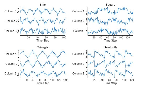
Visualize the first few sequences in plots.

figure tiledlayout(2,2) for i = 1:4 nexttile stackedplot(data{i})

xlabel("Time Step")
title(labels(i))

end

Prepare Data for Training

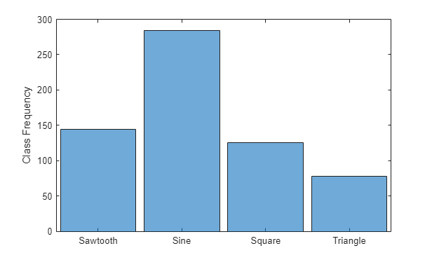
For class weights to affect training of a classification network, one or more classes must be more prevalent than others, in other words, the classes must be imbalanced. To demonstrate the effect of imbalanced classes for this example, retain all sine waves and remove approximately 30% of the sawtooth waves, 50% of the square waves, and 70% of the triangular waves.

idxImbalanced = (labels == "Sawtooth" & rand(numObservations,1) < 0.7)... | (labels == "Sine")... | (labels == "Square" & rand(numObservations,1) < 0.5)... | (labels == "Triangle" & rand(numObservations,1) < 0.3);

dataImbalanced = data(idxImbalanced); labelsImbalanced = labels(idxImbalanced);

View the balance of classes.

figure histogram(labelsImbalanced) ylabel("Class Frequency")

Set aside data for validation and testing. Using trainingPartitions, attached to this example as a supporting file, partition the data into a training set containing 70% of the data, a validation set containing 15% of the data, and a test set containing the remaining 15% of the data.

numObservations = numel(dataImbalanced);

[idxTrain, idxValidation, idxTest] = trainingPartitions(numObservations, [0.7 0.15 0.15]);

XTrain = dataImbalanced(idxTrain); XValidation = dataImbalanced(idxValidation); XTest = dataImbalanced(idxTest);

TTrain = labelsImbalanced(idxTrain); TValidation = labelsImbalanced(idxValidation); TTest = labelsImbalanced(idxTest);

Determine Inverse-Frequency Class Weights

For typical classification networks, a classification layer usually follows a softmax layer. During training, the classification layer calculates the cross-entropy loss by receiving values from the softmax layer and assigning each input value to one of K mutually exclusive classes using the cross-entropy function for a 1-of-K coding scheme [1]:

loss=1N∑n=1N∑i=1Kwitniln yni

N is the number of samples, K is the number of classes, wi is the weight for the class i, tni is the indicator that the nth sample belongs to the ith class, and yni is the value received from the softmax layer for sample n for class i. Classes with higher weights therefore contribute more to the loss.

To prevent the network being biased towards more prevalent classes, calculate class weights that are inversely proportional to the frequency of the classes:

wi=NK∑n=1Ntni

classes = unique(labelsImbalanced)'; for i=1:numClasses classFrequency(i) = sum(TTrain(:) == classes(i)); classWeights(i) = numel(XTrain)/(numClasses*classFrequency(i)); end

classes

classes = 1×4 categorical Sawtooth Sine Square Triangle

classWeights = 1×4

1.1276    0.5878    1.1162    1.9386

Define Network Architectures

Create a convolutional classification network.

Use a sequence input layer with an input size that matches the number of channels of the input data.
For a better fit and to prevent the training from diverging, set the Normalization option of the sequence input layer to "zscore". Doing so normalizes the sequence data to have zero mean and unit variance.
Use a 1-D convolution layer, a ReLU layer, and a batch normalization layer, where the convolution layer has 10 filters of width 10.
As the 1-D convolution layer requires that the input has at least as many time steps as the filter size, set the minimum length accepted by the sequence input layer equal to the filter size.
To help prevent the network from overfitting, specify a dropout layer.
To reduce the output of the convolution layer to a single vector, use a 1-D global max pooling layer.
To map the output to a vector of probabilities, specify a fully connected layer with an output size matching the number of classes.
Specify a softmax layer

filterSize = 10; numFilters = 10;

layers = [ ... sequenceInputLayer(numChannels,Normalization="zscore",MinLength=filterSize) convolution1dLayer(filterSize,numFilters) batchNormalizationLayer reluLayer dropoutLayer globalMaxPooling1dLayer fullyConnectedLayer(numClasses) softmaxLayer];

Specify Training Options

Specify the training options

Train using the Adam optimizer.
Train for 1000 epochs. For larger data sets, you might not need to train for as many epochs for a good fit.
Specify the sequences and classes used for validation.
Set the learning rate to 0.01.
Truncate the sequences in each mini-batch to have the same length as the shortest sequence. Truncating the sequences ensures that no padding is added, at the cost of discarding data. For sequences where all of the time steps in the sequence are likely to contain important information, truncation can prevent the network from achieving a good fit.
Output the network with the lowest validation loss.
Monitor the training progress in a plot and monitor the accuracy metric.
Disable the verbose output.

options = trainingOptions("adam", ... MaxEpochs=1000, ... ValidationData={XValidation, TValidation}, ... InitialLearnRate=0.01, ... SequenceLength="shortest", ... Verbose=false, ... Metrics="accuracy", ... Plots="training-progress");

Create a custom loss function that takes predictions Y and targets T and returns the weighted cross-entropy loss.

lossFcn = @(Y,T) crossentropy(Y,T,classWeights, ... NormalizationFactor="all-elements", ... WeightsFormat="C")*numClasses;

Train Networks

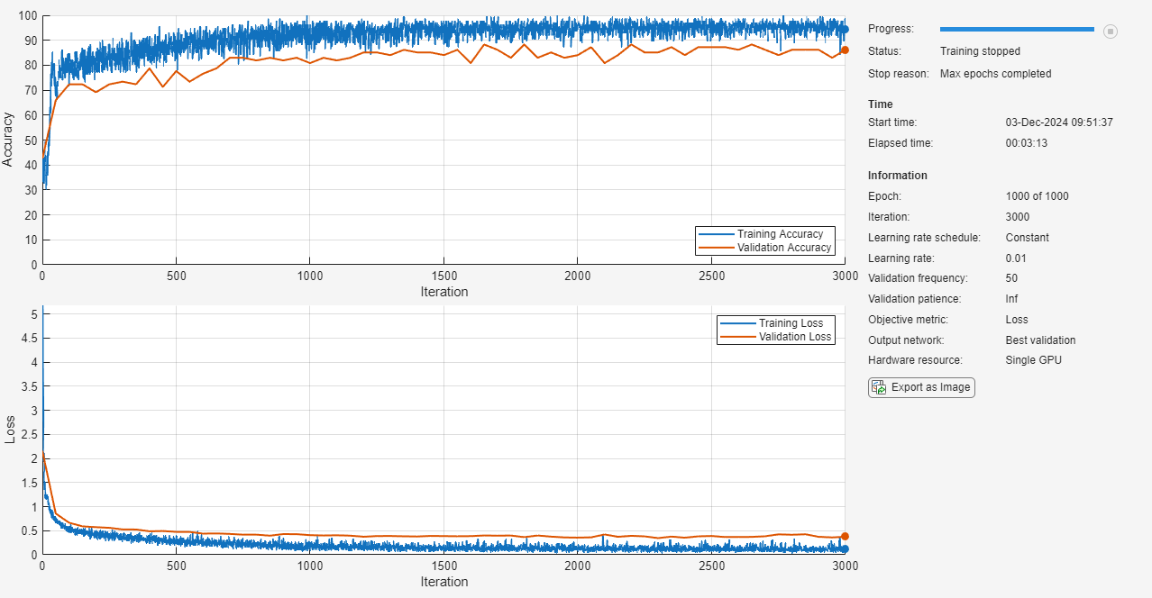
Train the convolutional networks with the specified options using the trainnet function.

netWeighted = trainnet(XTrain,TTrain,layers,lossFcn,options);

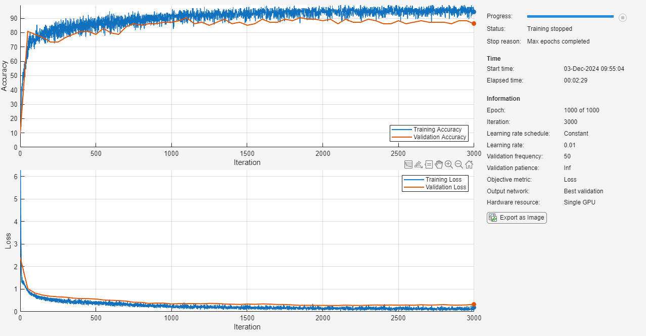
For comparison, train a second convolutional classification network that does not use class weights.

net = trainnet(XTrain,TTrain,layers,"crossentropy",options);

Compare Performance of Networks

Classify the test images. To make predictions with multiple observations, use the minibatchpredict function. To convert the prediction scores to labels, use the scores2label function. The minibatchpredict function automatically uses a GPU if one is available. Using a GPU requires a Parallel Computing Toolbox™ license and a supported GPU device. For information on supported devices, see GPU Computing Requirements (Parallel Computing Toolbox). Otherwise, the function uses the CPU.

scores = minibatchpredict(netWeighted,XTest); YWeighted = scores2label(scores,classes);

scores = minibatchpredict(net,XTest); Y = scores2label(scores,classes);

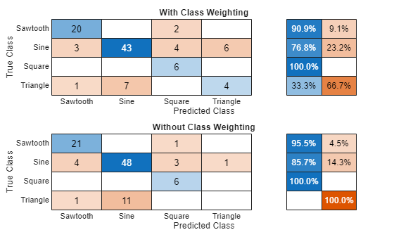
Visualize the predictions in confusion charts.

figure tiledlayout(2,1) nexttile CWeighted = confusionchart(TTest,YWeighted, ... Title="With Class Weighting", ... RowSummary="row-normalized"); nexttile C = confusionchart(TTest,Y, ... Title="Without Class Weighting", ... RowSummary="row-normalized");

Calculate the classification accuracy of the predictions.

accuracyWeighted = mean(YWeighted == TTest)

accuracyWeighted = 0.7604

accuracy = mean(Y == TTest)

In classification applications with imbalanced classes, accuracy can be a poor indicator of model performance. For example, a model can often achieve high accuracy by classifying every sample as the majority class.

Two other metrics for accessing model performance are precision (also known as the positive predictive value) and recall (also known as sensitivity).

Precision=True Positive True Positive+False Positive

Recall=True Positive True Positive+False Negative

To combine the precision and recall into a single metric, compute the F1-score [2]. The F1-score is commonly used for evaluating model performance.

F1=2(precision*recallprecision+recall)

A value close to 1 indicates that the model performs well.

You can monitor the precision, recall, or F1-score during training by specifying the Metrics training option as "precision", "recall" or "fscore". Or, you can monitor several metrics by specifying an array of metric names, such as ["accuracy" "fscore"]. By default, when you specify validation data, trainnet returns the network with the lowest validation loss. You can instead choose to return the network with the highest F1-score by specifying the ObjectiveMetricName option as "fscore". The objective metric does not change how a network trains. The objective metric only changes which network trainnet returns when training is complete.

Calculate the precision, recall, and F1-score for each class for both networks.

for i = 1:numClasses PrecisionWeighted(i) = CWeighted.NormalizedValues(i,i) / sum(CWeighted.NormalizedValues(i,:)); RecallWeighted(i) = CWeighted.NormalizedValues(i,i) / sum(CWeighted.NormalizedValues(:,i)); f1Weighted(i) = max(0,(2*PrecisionWeighted(i)*RecallWeighted(i)) / (PrecisionWeighted(i)+RecallWeighted(i))); end

for i = 1:numClasses Precision(i) = C.NormalizedValues(i,i) / sum(C.NormalizedValues(i,:)); Recall(i) = C.NormalizedValues(i,i) / sum(C.NormalizedValues(:,i)); f1(i) = max(0,(2*Precision(i)*Recall(i)) / (Precision(i)+Recall(i))); end

Calculate the average F1-score over all classes (macro-average) for both networks and visualize the F1-scores in a bar chart.

classesCombined = [classes "Macro-average"]; f1Combined = [f1 mean(f1); f1Weighted mean(f1Weighted)];

figure bar(classesCombined,f1Combined) ylim([0 1]) ylabel("F1-Score") legend("Without class weighting","With class weighting")

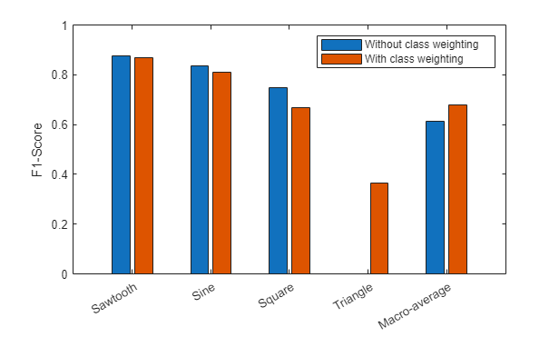
While weighting classes depending on frequency can decrease the overall accuracy of the predictions, doing so can improve the model's ability to classify less prevalent classes.

References

[1] Bishop, Christopher M. Pattern Recognition and Machine Learning. New York: Springer, 2006.

[2] Sokolova, Marina, and Guy Lapalme. "A Systematic Analysis of Performance Measures for Classification Tasks." Information Processing & Management 45, no. 4 (2009): 427–437.