Train Convolutional Neural Network for Regression - MATLAB & Simulink (original) (raw)
This example shows how to train a convolutional neural network to predict the angles of rotation of handwritten digits.
Regression tasks involve predicting continuous numerical values instead of discrete class labels. This example constructs a convolutional neural network architecture for regression, trains the network, and the uses the trained network to predict angles of rotated handwritten digits.
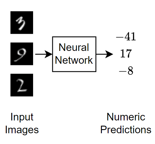
This diagram illustrates the flow of image data through a regression neural network.
Load Data
The data set contains synthetic images of handwritten digits together with the corresponding angles (in degrees) by which each image is rotated.
Load the training and test data from the MAT files DigitsDataTrain.mat and DigitsDataTest.mat, respectively. The variables anglesTrain and anglesTest are the rotation angles in degrees. The training and test data sets each contain 5000 images.
load DigitsDataTrain load DigitsDataTest
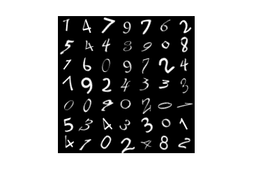
Display some of the training images.
numObservations = size(XTrain,4); idx = randperm(numObservations,49); I = imtile(XTrain(:,:,:,idx)); figure imshow(I);
Partition XTrain and anglesTrain into training and validation partitions using the trainingPartitions function, attached to this example as a supporting file. To access this function, open the example as a live script. Set aside 15% of the training data for validation.
[idxTrain,idxValidation] = trainingPartitions(numObservations,[0.85 0.15]);
XValidation = XTrain(:,:,:,idxValidation); anglesValidation = anglesTrain(idxValidation);
XTrain = XTrain(:,:,:,idxTrain); anglesTrain = anglesTrain(idxTrain);
Check Data Normalization
When training neural networks, it often helps to make sure that your data is normalized in all stages of the network. Normalization helps stabilize and speed up network training using gradient descent. If your data is poorly scaled, then the loss can become NaN and the network parameters can diverge during training. Common ways of normalizing data include rescaling the data so that its range becomes [0,1] or so that it has a mean of zero and standard deviation of one. You can normalize the following data:
- Input data. Normalize the predictors before you input them to the network. In this example, the input images are already normalized to the range [0,1].
- Layer outputs. You can normalize the outputs of each convolutional and fully connected layer by using a batch normalization layer.
- Responses. If you use batch normalization layers to normalize the layer outputs in the end of the network, then the predictions of the network are normalized when training starts. If the response has a very different scale from these predictions, then network training can fail to converge. If your response is poorly scaled, then try normalizing it and see if network training improves. If you normalize the response before training, then you must transform the predictions of the trained network to obtain the predictions of the original response.
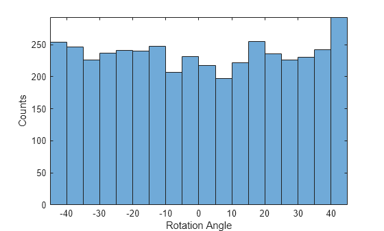
Plot the distribution of the response. The response (the rotation angle in degrees) is approximately uniformly distributed between -45 and 45, which works well without needing normalization. In classification problems, the outputs are class probabilities, which are always normalized.
figure histogram(anglesTrain) axis tight ylabel("Counts") xlabel("Rotation Angle")
In general, the data does not have to be exactly normalized. However, if you train the network in this example to predict 100*anglesTrain or anglesTrain+500 instead of anglesTrain, then the loss becomes NaN and the network parameters diverge when training starts. These results occur even though the only difference between a network predicting aY+b and a network predicting Y is a simple rescaling of the weights and biases of the final fully connected layer.
If the distribution of the input or response is very uneven or skewed, you can also perform nonlinear transformations (for example, taking logarithms) to the data before training the network.
Define Neural Network Architecture
Define the neural network architecture.
- For image input, specify an image input layer.
- Specify four convolution-batchnorm-ReLU blocks with increasing numbers of filters.
- Between each block, specify an average pooling layer with pooling regions and stride of size 2.
- At the end of the network, include a fully connected layer with an output size that matches the number of responses.
numResponses = 1;
layers = [ imageInputLayer([28 28 1]) convolution2dLayer(3,8,Padding="same") batchNormalizationLayer reluLayer averagePooling2dLayer(2,Stride=2) convolution2dLayer(3,16,Padding="same") batchNormalizationLayer reluLayer averagePooling2dLayer(2,Stride=2) convolution2dLayer(3,32,Padding="same") batchNormalizationLayer reluLayer convolution2dLayer(3,32,Padding="same") batchNormalizationLayer reluLayer fullyConnectedLayer(numResponses)];
Specify Training Options
Specify the training options. Choosing among the options requires empirical analysis. To explore different training option configurations by running experiments, you can use the Experiment Manager app.
- Set the initial learn rate to 0.001 and lower the learning rate after 20 epochs.
- Monitor the network accuracy during training by specifying validation data and validation frequency. The software trains the network on the training data and calculates the accuracy on the validation data at regular intervals during training. The validation data is not used to update the network weights.
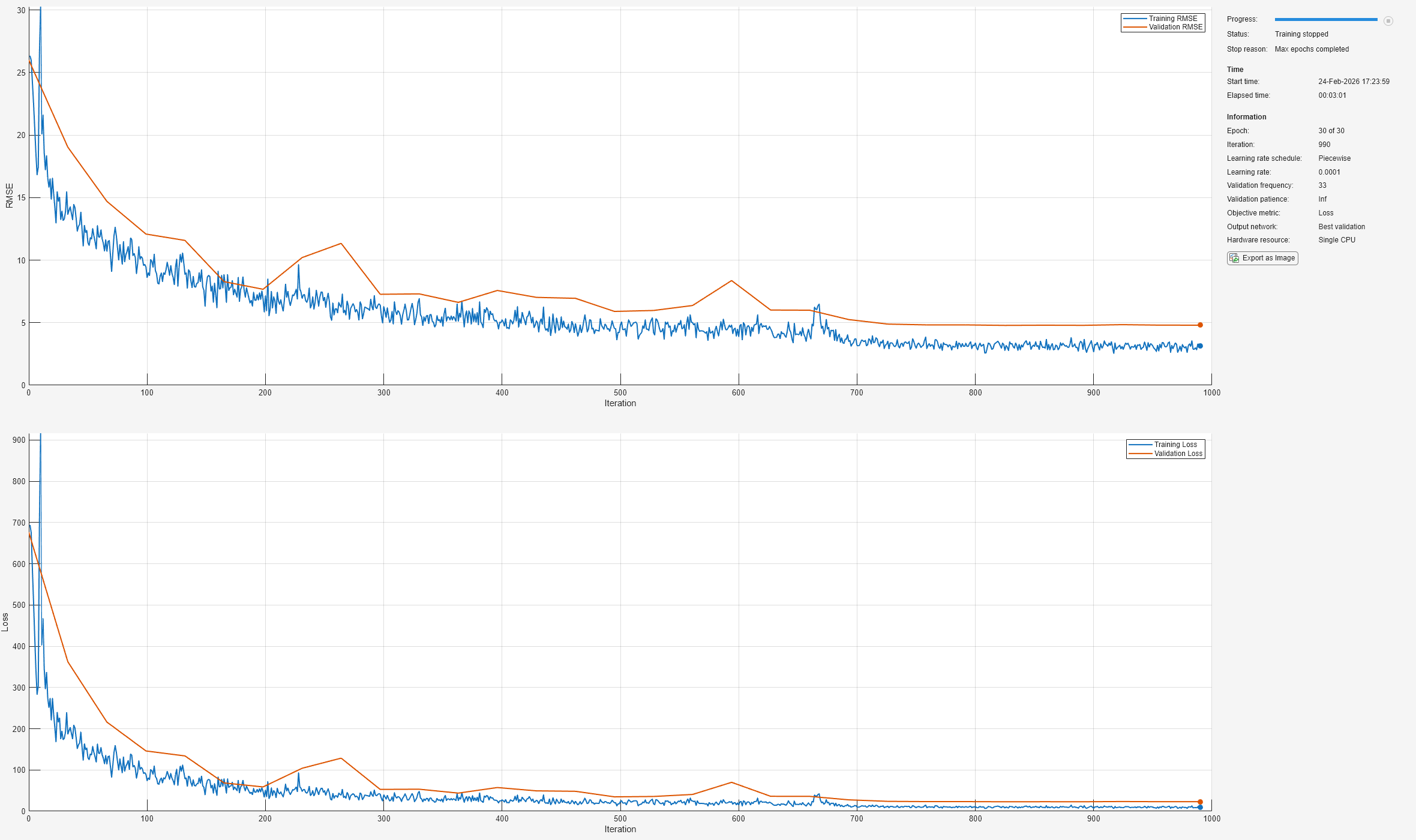
- Display the training progress in a plot and monitor the root mean squared error.
- Disable the verbose output.
miniBatchSize = 128; validationFrequency = floor(numel(anglesTrain)/miniBatchSize);
options = trainingOptions("sgdm", ... MiniBatchSize=miniBatchSize, ... InitialLearnRate=1e-3, ... LearnRateSchedule="piecewise", ... LearnRateDropFactor=0.1, ... LearnRateDropPeriod=20, ... Shuffle="every-epoch", ... ValidationData={XValidation,anglesValidation}, ... ValidationFrequency=validationFrequency, ... Plots="training-progress", ... Metrics="rmse", ... Verbose=false);
Train Neural Network
Train the neural network using the trainnet function. For regression, use mean squared error loss. By default, the trainnet function uses a GPU if one is available. Using a GPU requires a Parallel Computing Toolbox™ license and a supported GPU device. For information on supported devices, see GPU Computing Requirements (Parallel Computing Toolbox). Otherwise, the function uses the CPU. To specify the execution environment, use the ExecutionEnvironment training option.
net = trainnet(XTrain,anglesTrain,layers,"mse",options);
Test Network
Test the neural network using the testnet function. For regression, evaluate the root mean squared error (RMSE). By default, the testnet function uses a GPU if one is available. To select the execution environment manually, use the ExecutionEnvironment argument of the testnet function.
rmse = testnet(net,XTest,anglesTest,"rmse")
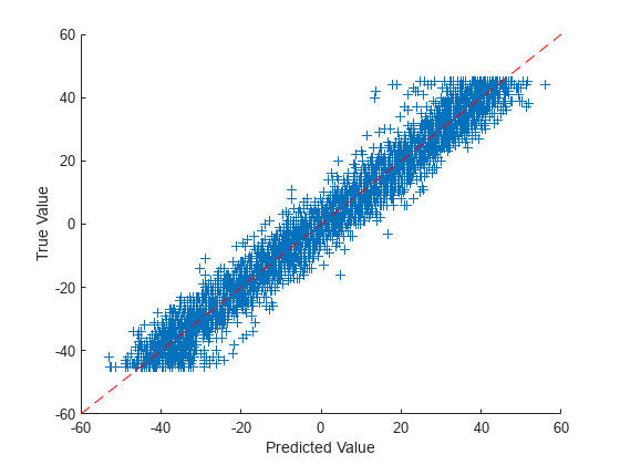
Visualize the accuracy in a plot by making predictions with the test data and comparing the predictions with the targets. Make predictions using the minibatchpredict function. By default, the minibatchpredict function uses a GPU if one is available.
YTest = minibatchpredict(net,XTest);
Plot the predicted values against the targets.
figure scatter(YTest,anglesTest,"+") xlabel("Prediction") ylabel("Target")
hold on plot([-60 60], [-60 60],"r--")
Make Predictions with New Data
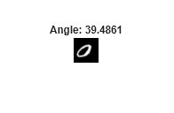
Use the neural network to make a prediction with the first test image. To make a prediction with a single image, use the predict function. To use a GPU, first convert the data to gpuArray.
X = XTest(:,:,:,1); if canUseGPU X = gpuArray(X); end Y = predict(net,X)
figure imshow(X) title("Angle: " + gather(Y))
See Also
trainnet | trainingOptions | dlnetwork