Create a Deep Learning Experiment for Regression - MATLAB & Simulink (original) (raw)
Main Content
This example shows how to train a deep learning network for regression by using Experiment Manager. In this example, you use a regression model to predict the angles of rotation of handwritten digits. A custom metric function determines the fraction of angle predictions within an acceptable error margin from the true angles. For more information on using a regression model, see Train Convolutional Neural Network for Regression.
Open Experiment
First, open the example. Experiment Manager loads a project with a preconfigured experiment that you can inspect and run. To open the experiment, in the Experiment Browser pane, double-click RegressionExperiment.

Built-in training experiments consist of a description, a table of hyperparameters, a setup function, and a collection of metric functions to evaluate the results of the experiment. For more information, see Train Network Using trainnet and Display Custom Metrics.
The Description field contains a textual description of the experiment. For this example, the description is:
Regression model to predict angles of rotation of digits, using hyperparameters to specify:
- the number of filters used by the convolution layers
- the probability of the dropout layer in the network
The Hyperparameters section specifies the strategy and hyperparameter values to use for the experiment. When you run the experiment, Experiment Manager trains the network using every combination of hyperparameter values specified in the hyperparameter table. This example uses two hyperparameters:
Probabilitysets the probability of the dropout layer in the neural network. By default, the values for this hyperparameter are specified as[0.1 0.2].Filtersindicates the number of filters used by the first convolution layer in the neural network. In the subsequent convolution layers, the number of filters is a multiple of this value. By default, the values of this hyperparameter are specified as[4 6 8].
The Setup Function section specifies a function that configures the training data, network architecture, and training options for the experiment. To open this function in MATLAB® Editor, click Edit. The code for the function also appears in Setup Function. The input to the setup function is a structure with fields from the hyperparameter table. The function returns four outputs that you use to train a network for image regression problems. In this example, the setup function has these sections:
- Load Training Data defines the training and validation data for the experiment as 4-D arrays. The training and validation data sets each contain 5000 images of digits from 0 to 9. The regression values correspond to the angles of rotation of the digits.
[XTrain,,YTrain] = digitTrain4DArrayData;
[XValidation,,YValidation] = digitTest4DArrayData;
- Define Network Architecture defines the architecture for a convolutional neural network for regression.
inputSize = [28 28 1]; numFilters = params.Filters;
layers = [ imageInputLayer(inputSize)
convolution2dLayer(3,numFilters,Padding="same")
batchNormalizationLayer
reluLayer

averagePooling2dLayer(2,Stride=2)

convolution2dLayer(3,2*numFilters,Padding="same")
batchNormalizationLayer
reluLayer

averagePooling2dLayer(2,Stride=2)

convolution2dLayer(3,4*numFilters,Padding="same")
batchNormalizationLayer
reluLayer

convolution2dLayer(3,4*numFilters,Padding="same")
batchNormalizationLayer
reluLayer

dropoutLayer(params.Probability)
fullyConnectedLayer(1)
regressionLayer];- Specify Training Options defines a trainingOptions object for the experiment. The example trains the network for 30 epochs. The learning rate is initially 0.001 and drops by a factor of 0.1 after 20 epochs. The software trains the network on the training data and calculates the root mean squared error (RMSE) and loss on the validation data at regular intervals during training. The validation data is not used to update the network weights.
miniBatchSize = 128; validationFrequency = floor(numel(YTrain)/miniBatchSize); options = trainingOptions("sgdm", ... MiniBatchSize=miniBatchSize, ... MaxEpochs=30, ... InitialLearnRate=1e-3, ... LearnRateSchedule="piecewise", ... LearnRateDropFactor=0.1, ... LearnRateDropPeriod=20, ... Shuffle="every-epoch", ... ValidationData={XValidation,YValidation}, ... ValidationFrequency=validationFrequency, ... Verbose=false);
The Metrics section specifies optional functions that evaluate the results of the experiment. Experiment Manager evaluates these functions each time it finishes training the network. This example includes a metric function Accuracy that determines the percentage of angle predictions within an acceptable error margin from the true angles. By default, the function uses a threshold of 10 degrees. To open this function in MATLAB Editor, select the name of the metric function and click Edit. The code for the function also appears in Compute Accuracy of Regression Model.
Run Experiment
When you run the experiment, Experiment Manager trains the network defined by the setup function six times. Each trial uses a different combination of hyperparameter values. By default, Experiment Manager runs one trial at a time. If you have Parallel Computing Toolbox™, you can run multiple trials at the same time or offload your experiment as a batch job in a cluster:
- To run one trial of the experiment at a time, on the Experiment Manager toolstrip, set Mode to
Sequentialand click Run. - To run multiple trials at the same time, set Mode to
Simultaneousand click Run. If there is no current parallel pool, Experiment Manager starts one using the default cluster profile. Experiment Manager then runs as many simultaneous trials as there are workers in your parallel pool. For best results, before you run your experiment, start a parallel pool with as many workers as GPUs. For more information, see Run Experiments in Parallel and GPU Computing Requirements (Parallel Computing Toolbox). - To offload the experiment as a batch job, set Mode to
Batch SequentialorBatch Simultaneous, specify your cluster and pool size, and click Run. For more information, see Offload Experiments as Batch Jobs to a Cluster.
A table of results displays the RMSE and loss for each trial. The table also displays the accuracy of the trial, as determined by the custom metric function Accuracy.

To display the training plot and track the progress of each trial while the experiment is running, under Review Results, click Training Plot.

Evaluate Results
To find the best result for your experiment, sort the table of results by accuracy:
- Point to the Accuracy column.
- Click the triangle icon.
- Select Sort in Descending Order.
The trial with the highest accuracy appears at the top of the results table.

To test the performance of an individual trial, export the trained network and display a box plot of the residuals for each digit class:
- Select the trial with the highest accuracy.
- On the Experiment Manager toolstrip, click Export > Trained Network.
- In the dialog window, enter the name of a workspace variable for the exported network. The default name is
trainedNetwork. - In the MATLAB Command Window, use the exported network as the input to the function
plotResiduals:
plotResiduals(trainedNetwork)
To view the code for this function, see Display Box Plot of Residuals for Each Digit. The function creates a residual box plot for each digit. The digit classes with highest accuracy have a mean close to zero and little variance.

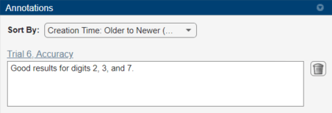
To record observations about the results of your experiment, add an annotation:
- In the results table, right-click the Accuracy cell of the best trial.
- Select Add Annotation.
- In the Annotations pane, enter your observations in the text box.
Close Experiment
In the Experiment Browser pane, right-click DigitRegressionWithAccuracyProject and select Close Project. Experiment Manager closes the experiment and results contained in the project.
Setup Function
This function configures the training data, network architecture, and training options for the experiment. The input to this function is a structure with fields from the hyperparameter table. The function returns four outputs that you use to train a network for image regression problems.
function [XTrain,YTrain,layers,options] = RegressionExperiment_setup(params)
Load Training Data
[XTrain,,YTrain] = digitTrain4DArrayData;
[XValidation,,YValidation] = digitTest4DArrayData;
Define Network Architecture
inputSize = [28 28 1]; numFilters = params.Filters;
layers = [ imageInputLayer(inputSize)
convolution2dLayer(3,numFilters,Padding="same")
batchNormalizationLayer
reluLayer

averagePooling2dLayer(2,Stride=2)

convolution2dLayer(3,2*numFilters,Padding="same")
batchNormalizationLayer
reluLayer

averagePooling2dLayer(2,Stride=2)

convolution2dLayer(3,4*numFilters,Padding="same")
batchNormalizationLayer
reluLayer

convolution2dLayer(3,4*numFilters,Padding="same")
batchNormalizationLayer
reluLayer

dropoutLayer(params.Probability)
fullyConnectedLayer(1)
regressionLayer];
Specify Training Options
miniBatchSize = 128; validationFrequency = floor(numel(YTrain)/miniBatchSize); options = trainingOptions("sgdm", ... MiniBatchSize=miniBatchSize, ... MaxEpochs=30, ... InitialLearnRate=1e-3, ... LearnRateSchedule="piecewise", ... LearnRateDropFactor=0.1, ... LearnRateDropPeriod=20, ... Shuffle="every-epoch", ... ValidationData={XValidation,YValidation}, ... ValidationFrequency=validationFrequency, ... Verbose=false);
Compute Accuracy of Regression Model
This metric function calculates the number of predictions within an acceptable error margin from the true angles.
function metricOutput = Accuracy(trialInfo)
[XValidation,~,YValidation] = digitTest4DArrayData; YPredicted = predict(trialInfo.trainedNetwork,XValidation); predictionError = YValidation - YPredicted;
thr = 10; numCorrect = sum(abs(predictionError) < thr); numValidationImages = numel(YValidation);
metricOutput = 100*numCorrect/numValidationImages; end
Display Box Plot of Residuals for Each Digit
This function creates a residual box plot for each digit.
function plotResiduals(net)
[XValidation,~,YValidation] = digitTest4DArrayData; YPredicted = predict(net,XValidation); predictionError = YValidation - YPredicted; residualMatrix = reshape(predictionError,500,10);
figure boxplot(residualMatrix,... "Labels",["0","1","2","3","4","5","6","7","8","9"]) xlabel("Digit Class") ylabel("Degrees Error") title("Residuals") end