Add Event Table from External Data to Timetable - MATLAB & Simulink (original) (raw)
To find and label events in a timetable, attach an eventtable to it. An event table is a timetable of events. An event consists of an event time (when something happened), often an event length or event end time (how long it happened), often an event label (what happened), and sometimes additional information about the event. When you attach an event table to a timetable, it enables you to find and label rows in the timetable that occur during events. By associating timetable rows with events, you can more easily analyze and plot the data that they contain.
This example shows how you can add events to your timetable using data that comes from an external data source. In the example, import a timetable of measurements of the Earth's rotation rate from 1962 to the present. The rotation rate varies as a function of time, causing changes in the excess length-of-day to accumulate. Whenever the cumulative excess becomes too large, a leap second is inserted. This example analyzes the excess length-of-day over time and treats leap seconds added since 1972 as a set of external events. To analyze these data with event tables, use the eventtable, eventfilter, and syncevents functions. (A related workflow is to find and label events within your timetable. For more information about that workflow, see Find Events in Timetable Using Event Table.)
Import Timetable with Length-of-Day Measurements
By definition, a day is 86,400 seconds long, where the second has a precise definition in the International System of Units (SI). However, the length of a day actually varies due to several physical causes. It varies with the seasons by as much as 30 seconds over and 21 seconds under the SI definition because of the eccentricity of Earth's orbit and the tilt of its axis. Averaging these seasonal effects enables the definition of the mean solar day, which does not vary in length over a year.
Also, there is a very long-term slowing in the rotational speed of the Earth due to tidal interaction with the moon; a smaller, opposite, shorter-term component believed to be due to melting of continental ice sheets; very short-term cycles on the order of decades; and unpredictable fluctuations due to geological events and other causes. Because of those effects, the length of a mean solar day might increase or decrease. In recent decades, it has fluctuated up and down, but has mostly been 1–3 milliseconds longer than 86,400 seconds. That difference is known as the excess Length of Day, or excess LOD.
For this example, create a timetable that contains the excess LOD for every day from January 1, 1962, to the present. The International Earth Rotation and Reference Systems Service (IERS) collects and publishes this data. However, this data needs preprocessing before storing in a MATLAB timetable because the dates are modified Julian dates. To read the IERS data into a table, use the readtable function. Rename the two variables of interest to MJD and ExcessLOD.
file = "https://datacenter.iers.org/data/latestVersion/223_EOP_C04_14.62-NOW.IAU1980223.txt"; IERSdata = readtable(file,NumHeaderLines=14); IERSdata.Properties.VariableNames([4 8]) = ["MJD","ExcessLOD"];
To store the excess LOD values in a timetable, convert the modified Julian dates to datetime values. Use the datetime function with the ConvertFrom="mjd" name-value argument. Convert the excess LOD values to duration values by using the seconds function. Then convert IERSdata from a table to a timetable using the table2timetable function.
IERSdata.Date = datetime(IERSdata.MJD,ConvertFrom="mjd"); IERSdata.ExcessLOD = seconds(IERSdata.ExcessLOD); IERSdata = table2timetable(IERSdata(:,["Date","ExcessLOD"]))
IERSdata=22458×1 timetable
Date ExcessLOD
___________ ____________
01-Jan-1962 0.001723 sec
02-Jan-1962 0.001669 sec
03-Jan-1962 0.001582 sec
04-Jan-1962 0.001496 sec
05-Jan-1962 0.001416 sec
06-Jan-1962 0.001382 sec
07-Jan-1962 0.001413 sec
08-Jan-1962 0.001505 sec
09-Jan-1962 0.001628 sec
10-Jan-1962 0.001738 sec
11-Jan-1962 0.001794 sec
12-Jan-1962 0.001774 sec
13-Jan-1962 0.001667 sec
14-Jan-1962 0.00151 sec
15-Jan-1962 0.001312 sec
16-Jan-1962 0.001112 sec
⋮
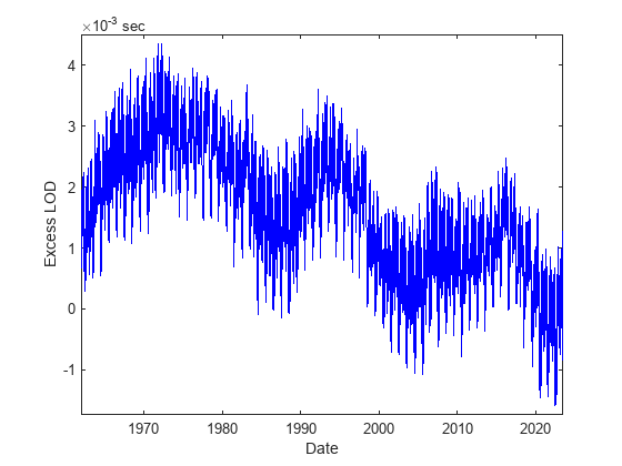
Plot the excess LOD as a function of time. The excess LOD is currently decreasing on average but has remained positive except during very brief periods.
plot(IERSdata.Date,IERSdata.ExcessLOD,"b-"); xlabel("Date"); ylabel("Excess LOD");
Calculate Cumulative Excess Length of Day
A clock that defines a day as 86,400 SI seconds is effectively running fast with respect to the Earth's rotation, gaining time with respect to the sun each day. A few extra milliseconds per day might seem unimportant, but the excess LOD since 1962 accumulates.
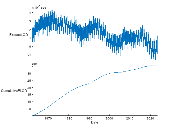
Add the cumulative excess LOD to IERSdata as another table variable. To calculate the cumulative sum of the excess LOD, use the cumsum function. Then use the stackedplot function to plot excess LOD and cumulative excess LOD together. This plot shows that the shift due to the accumulated excess LOD since the 1960s has been less than one minute.
IERSdata.CumulativeELOD = [0; cumsum(IERSdata.ExcessLOD(1:end-1))]; stackedplot(IERSdata,["ExcessLOD","CumulativeELOD"])
Store Leap Seconds in Event Table
At midnight on January 1, 1972, the current version of the system of time known as Coordinated Universal Time (UTC) was enacted, which uses 86,400 SI seconds per day. On that date, UTC was defined to be roughly in sync with solar time at the Greenwich Meridian, or more precisely, with the time known as UT1. However, timekeeping based on exactly 86,400 SI seconds per day would drift away from our physical experience of solar time because of accumulated excess LOD. So, when needed, an extra leap second adjustment is inserted to keep UTC approximately in sync with solar time. Without these leap second adjustments after 1972, accumulated excess LOD would have caused UTC to drift away from UT1 over the years. Within decades, the difference would have grown to tens of seconds.
Show the difference since 1972. First, select the post-1971 excess LOD data by subscripting into IERSdata with a time range starting on January 1, 1972. To create that time range, use the timerange function.
IERSdata1972 = IERSdata(timerange("1972-01-01",Inf),"ExcessLOD")
IERSdata1972=18806×1 timetable
Date ExcessLOD
___________ ____________
01-Jan-1972 0.002539 sec
02-Jan-1972 0.002708 sec
03-Jan-1972 0.002897 sec
04-Jan-1972 0.003065 sec
05-Jan-1972 0.003177 sec
06-Jan-1972 0.00322 sec
07-Jan-1972 0.003201 sec
08-Jan-1972 0.003137 sec
09-Jan-1972 0.003033 sec
10-Jan-1972 0.002898 sec
11-Jan-1972 0.002772 sec
12-Jan-1972 0.002672 sec
13-Jan-1972 0.002621 sec
14-Jan-1972 0.002642 sec
15-Jan-1972 0.00274 sec
16-Jan-1972 0.002937 sec
⋮
Add another variable with the unadjusted difference since 1972. Start with the cumulative excess LOD on January 1, 1972, which was 0.0454859 second. For every date that follows, calculate the unadjusted difference. By the beginning of 2017, the unadjusted difference would have grown to about 26 seconds. Display IERSdata1972 using a time range that includes the start of 2017.
DiffUT1_1972 = seconds(0.0454859); IERSdata1972.UnadjustedDiff = DiffUT1_1972 + [0; cumsum(IERSdata1972.ExcessLOD(1:end-1))]; IERSdata1972(timerange("2016-12-29","2017-01-04"),:)
ans=6×2 timetable
Date ExcessLOD UnadjustedDiff
___________ _____________ ______________
29-Dec-2016 0.0008055 sec 26.402 sec
30-Dec-2016 0.0008525 sec 26.402 sec
31-Dec-2016 0.0009173 sec 26.403 sec
01-Jan-2017 0.001016 sec 26.404 sec
02-Jan-2017 0.0011845 sec 26.405 sec
03-Jan-2017 0.0013554 sec 26.406 sec
This drift is what leap seconds are designed to mitigate. You can think of each leap second that is inserted into the UTC timeline as an event. These events are not part of the LOD data. However, in MATLAB the leapseconds function lists each leap second that has occurred since 1972. (The leap seconds listed by leapseconds come from another data set provided by the IERS.) The timetable returned by leapseconds contains a timestamp, a description of each event (+ for leap second insertions, - for removals), and the cumulative number of leap seconds up to and including the event. To date, there have been 27 leap second events, and they have all been insertions.
lsEvents=27×2 timetable
Date Type CumulativeAdjustment
___________ ____ ____________________
30-Jun-1972 + 1 sec
31-Dec-1972 + 2 sec
31-Dec-1973 + 3 sec
31-Dec-1974 + 4 sec
31-Dec-1975 + 5 sec
31-Dec-1976 + 6 sec
31-Dec-1977 + 7 sec
31-Dec-1978 + 8 sec
31-Dec-1979 + 9 sec
30-Jun-1981 + 10 sec
30-Jun-1982 + 11 sec
30-Jun-1983 + 12 sec
30-Jun-1985 + 13 sec
31-Dec-1987 + 14 sec
31-Dec-1989 + 15 sec
31-Dec-1990 + 16 sec
⋮
To treat the leap seconds as events, convert lsEvents to an event table by using the eventtable function.
lsEvents = eventtable(lsEvents)
lsEvents = 27×2 eventtable
Event Labels Variable:
Event Lengths Variable:
Date Type CumulativeAdjustment
___________ ____ ____________________
30-Jun-1972 + 1 sec
31-Dec-1972 + 2 sec
31-Dec-1973 + 3 sec
31-Dec-1974 + 4 sec
31-Dec-1975 + 5 sec
31-Dec-1976 + 6 sec
31-Dec-1977 + 7 sec
31-Dec-1978 + 8 sec
31-Dec-1979 + 9 sec
30-Jun-1981 + 10 sec
30-Jun-1982 + 11 sec
30-Jun-1983 + 12 sec
30-Jun-1985 + 13 sec
31-Dec-1987 + 14 sec
31-Dec-1989 + 15 sec
31-Dec-1990 + 16 sec
30-Jun-1992 + 17 sec
30-Jun-1993 + 18 sec
30-Jun-1994 + 19 sec
31-Dec-1995 + 20 sec
30-Jun-1997 + 21 sec
31-Dec-1998 + 22 sec
31-Dec-2005 + 23 sec
31-Dec-2008 + 24 sec
30-Jun-2012 + 25 sec
30-Jun-2015 + 26 sec
31-Dec-2016 + 27 sec
At this point, the main LOD data is in the IERSdata1972 timetable. The leap second events are in the lsEvents event table. To find and label rows that occur during leap seconds in the LOD data, attach lsEvents to IERSdata1972. Assign lsEvents to its Events property.
IERSdata1972.Properties.Events = lsEvents; IERSdata1972.Properties
ans = TimetableProperties with properties: Description: '' UserData: [] DimensionNames: {'Date' 'Variables'} VariableNames: {'ExcessLOD' 'UnadjustedDiff'} VariableDescriptions: {} VariableUnits: {} VariableContinuity: [] RowTimes: [18806×1 datetime] StartTime: 01-Jan-1972 SampleRate: NaN TimeStep: 1d Events: [27×2 eventtable] CustomProperties: No custom properties are set. Use addprop and rmprop to modify CustomProperties.
Use Event Timestamps to Select Data
Add the unadjusted difference, or cumulative excess LOD, at each date in lsEvents. To find the unadjusted differences on these dates, index into the UnadjustedDiff variable of IERSdata1972 and select the unadjusted difference at the timestamps from lsEvents. Then append those differences to each event in lsEvents as additional information about the event.
First, create an event filter using the eventfilter function. It uses the event table attached to a timetable to create a row subscript. You can use subscript into timetables rows using matching values from the event table. Subscript into IERSdata1972 and return an array of unadjusted differences on the dates when leap seconds were added.
EF = eventfilter(IERSdata1972)
EF = eventfilter with no constraints and no selected variables
<unconstrained>VariableNames: Date, Type, CumulativeAdjustment
UnadjustedDiff = IERSdata1972{EF.Date,"UnadjustedDiff"}
UnadjustedDiff = 27×1 duration 0.63494 sec 1.1864 sec 2.2976 sec 3.289 sec 4.2718 sec 5.3334 sec 6.3469 sec 7.398 sec 8.3526 sec 9.6281 sec 10.389 sec 11.249 sec 12.451 sec 13.634 sec 14.669 sec 15.379 sec 16.556 sec 17.399 sec 18.216 sec 19.442 sec 20.472 sec 21.282 sec 22.659 sec 23.589 sec 24.583 sec 25.671 sec 26.403 sec
Add the array as a new variable to the event table. In this way, you can add more information about events after you have attached an event table to a timetable.
IERSdata1972.Properties.Events.UnadjustedDiff = UnadjustedDiff
IERSdata1972=18806×2 timetable Date ExcessLOD UnadjustedDiff ___________ ____________ ______________ 01-Jan-1972 0.002539 sec 0.045486 sec 02-Jan-1972 0.002708 sec 0.048025 sec 03-Jan-1972 0.002897 sec 0.050733 sec 04-Jan-1972 0.003065 sec 0.05363 sec 05-Jan-1972 0.003177 sec 0.056695 sec 06-Jan-1972 0.00322 sec 0.059872 sec 07-Jan-1972 0.003201 sec 0.063092 sec 08-Jan-1972 0.003137 sec 0.066293 sec 09-Jan-1972 0.003033 sec 0.06943 sec 10-Jan-1972 0.002898 sec 0.072463 sec 11-Jan-1972 0.002772 sec 0.075361 sec 12-Jan-1972 0.002672 sec 0.078133 sec 13-Jan-1972 0.002621 sec 0.080805 sec 14-Jan-1972 0.002642 sec 0.083426 sec 15-Jan-1972 0.00274 sec 0.086068 sec 16-Jan-1972 0.002937 sec 0.088808 sec ⋮
Plot Events Against Data
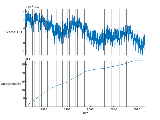
The event table shows that at each event, the IERS inserted a leap second whenever the excess LOD accumulated by roughly one additional second. To confirm this observation visually, plot the LOD data overlaid with the instantaneous leap second events. Use the stackedplot function. If the input is a timetable with an attached event table, then stackedplot automatically plots events from the event table on top of the data from the timetable. It plots instantaneous events as vertical lines.
stackedplot(IERSdata1972)
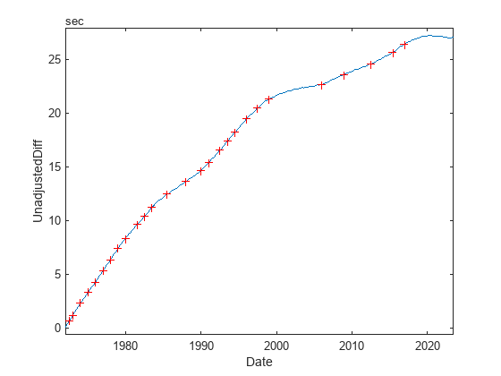
The stackedplot function plots all events using the same default style. To plot events using different styles, use the plot function and specify colors, markers, line styles, and so on. For example, plot the leap second events on the unadjusted differences using red crosses instead of vertical lines.
plot(IERSdata1972,"UnadjustedDiff"); hold on plot(lsEvents.Date,IERSdata1972.UnadjustedDiff(lsEvents.Date),"r+"); hold off
Copy Event Data to State Variable in Timetable
The leap seconds are instantaneous events recorded in an event table. Another way to represent them is by using a state variable appended to the original LOD data. A state variable describes the "state" of the process being measured at each time point rather than tagging a specific instant. One possible state variable for this leap second data is an indicator variable that records an adjustment on each event date, with missing values on all the other dates. This approach works because all timestamps from the event table are also timestamps in IERSdata1972.
To copy the cumulative adjustments from the attached event table to the timetable, use the syncevents function. The function automatically fills the other elements of the new CumulativeAdjustment variable with missing values. Display the timetable rows around the 27th leap second.
IERSdata1972 = syncevents(IERSdata1972,EventDataVariables="CumulativeAdjustment"); IERSdata1972(timerange("2016-12-29","2017-01-04"),:)
ans=6×3 timetable
Date ExcessLOD UnadjustedDiff CumulativeAdjustment
___________ _____________ ______________ ____________________
29-Dec-2016 0.0008055 sec 26.402 sec NaN sec
30-Dec-2016 0.0008525 sec 26.402 sec NaN sec
<1 event> 31-Dec-2016 0.0009173 sec 26.403 sec 27 sec
01-Jan-2017 0.001016 sec 26.404 sec NaN sec
02-Jan-2017 0.0011845 sec 26.405 sec NaN sec
03-Jan-2017 0.0013554 sec 26.406 sec NaN sec
Another possibility, more useful in this example, is to add a state variable that indicates the cumulative sum of leap seconds at any given date in the LOD data. Begin by removing the CumulativeAdjustment variable from the timetable.
IERSdata1972.CumulativeAdjustment = []; % remove the previous state variable
Then assign the attached event table to local variable in the workspace.
lsEvents = IERSdata1972.Properties.Events;
The data in IERSdata1972 begin on January 1, 1972, before the first leap second was added. So, add one more event to lsEvents, to cover the time before the first leap second.
lsEvents(IERSdata1972.Date(1),:) = {"+",seconds(0),seconds(0)}; lsEvents = sortrows(lsEvents)
lsEvents = 28×3 eventtable
Event Labels Variable:
Event Lengths Variable:
Date Type CumulativeAdjustment UnadjustedDiff
___________ ____ ____________________ ______________
01-Jan-1972 + 0 sec 0 sec
30-Jun-1972 + 1 sec 0.63494 sec
31-Dec-1972 + 2 sec 1.1864 sec
31-Dec-1973 + 3 sec 2.2976 sec
31-Dec-1974 + 4 sec 3.289 sec
31-Dec-1975 + 5 sec 4.2718 sec
31-Dec-1976 + 6 sec 5.3334 sec
31-Dec-1977 + 7 sec 6.3469 sec
31-Dec-1978 + 8 sec 7.398 sec
31-Dec-1979 + 9 sec 8.3526 sec
30-Jun-1981 + 10 sec 9.6281 sec
30-Jun-1982 + 11 sec 10.389 sec
30-Jun-1983 + 12 sec 11.249 sec
30-Jun-1985 + 13 sec 12.451 sec
31-Dec-1987 + 14 sec 13.634 sec
31-Dec-1989 + 15 sec 14.669 sec
31-Dec-1990 + 16 sec 15.379 sec
30-Jun-1992 + 17 sec 16.556 sec
30-Jun-1993 + 18 sec 17.399 sec
30-Jun-1994 + 19 sec 18.216 sec
31-Dec-1995 + 20 sec 19.442 sec
30-Jun-1997 + 21 sec 20.472 sec
31-Dec-1998 + 22 sec 21.282 sec
31-Dec-2005 + 23 sec 22.659 sec
31-Dec-2008 + 24 sec 23.589 sec
30-Jun-2012 + 25 sec 24.583 sec
30-Jun-2015 + 26 sec 25.671 sec
31-Dec-2016 + 27 sec 26.403 sec
Add event end times to transform the events into interval events. The end of each interval is the day before the next leap second was added. The last event end time is the last date in IERSdata1972.
endEvents = [lsEvents.Date(2:end) - 1 ; IERSdata1972.Date(end)];
Add the event end times to lsEvents as a new variable. Then assign the new variable to the EventEndsVariable property of lsEvents. Event tables have properties that specify which of their variables contain event labels, event lengths, or event end times.
lsEvents.EventEnds = endEvents; lsEvents.Properties.EventEndsVariable = "EventEnds"
lsEvents = 28×4 eventtable Event Labels Variable: Event Ends Variable: EventEnds Date Type CumulativeAdjustment UnadjustedDiff EventEnds ___________ ____ ____________________ ______________ ___________ 01-Jan-1972 + 0 sec 0 sec 29-Jun-1972 30-Jun-1972 + 1 sec 0.63494 sec 30-Dec-1972 31-Dec-1972 + 2 sec 1.1864 sec 30-Dec-1973 31-Dec-1973 + 3 sec 2.2976 sec 30-Dec-1974 31-Dec-1974 + 4 sec 3.289 sec 30-Dec-1975 31-Dec-1975 + 5 sec 4.2718 sec 30-Dec-1976 31-Dec-1976 + 6 sec 5.3334 sec 30-Dec-1977 31-Dec-1977 + 7 sec 6.3469 sec 30-Dec-1978 31-Dec-1978 + 8 sec 7.398 sec 30-Dec-1979 31-Dec-1979 + 9 sec 8.3526 sec 29-Jun-1981 30-Jun-1981 + 10 sec 9.6281 sec 29-Jun-1982 30-Jun-1982 + 11 sec 10.389 sec 29-Jun-1983 30-Jun-1983 + 12 sec 11.249 sec 29-Jun-1985 30-Jun-1985 + 13 sec 12.451 sec 30-Dec-1987 31-Dec-1987 + 14 sec 13.634 sec 30-Dec-1989 31-Dec-1989 + 15 sec 14.669 sec 30-Dec-1990 31-Dec-1990 + 16 sec 15.379 sec 29-Jun-1992 30-Jun-1992 + 17 sec 16.556 sec 29-Jun-1993 30-Jun-1993 + 18 sec 17.399 sec 29-Jun-1994 30-Jun-1994 + 19 sec 18.216 sec 30-Dec-1995 31-Dec-1995 + 20 sec 19.442 sec 29-Jun-1997 30-Jun-1997 + 21 sec 20.472 sec 30-Dec-1998 31-Dec-1998 + 22 sec 21.282 sec 30-Dec-2005 31-Dec-2005 + 23 sec 22.659 sec 30-Dec-2008 31-Dec-2008 + 24 sec 23.589 sec 29-Jun-2012 30-Jun-2012 + 25 sec 24.583 sec 29-Jun-2015 30-Jun-2015 + 26 sec 25.671 sec 30-Dec-2016 31-Dec-2016 + 27 sec 26.403 sec 27-Jun-2023
Attach lsEvents to IERSdata1972.
IERSdata1972.Properties.Events = lsEvents;
Copy the cumulative adjustments by calling syncevents. The attached event table has interval events, so syncevents fills in every row of IERSdata1972 with event data that occurs during the intervals. Every row of IERSdata1972 records the cumulative adjustment that occurred up to that time.
IERSdata1972 = syncevents(IERSdata1972,EventDataVariables="CumulativeAdjustment"); IERSdata1972(timerange("2016-12-29","2017-01-04"),:)
ans=6×3 timetable
Date ExcessLOD UnadjustedDiff CumulativeAdjustment
___________ _____________ ______________ ____________________
<1 event> 29-Dec-2016 0.0008055 sec 26.402 sec 26 sec
30-Dec-2016 0.0008525 sec 26.402 sec NaN sec
<1 event> 31-Dec-2016 0.0009173 sec 26.403 sec 27 sec
<1 event> 01-Jan-2017 0.001016 sec 26.404 sec 27 sec
<1 event> 02-Jan-2017 0.0011845 sec 26.405 sec 27 sec
<1 event> 03-Jan-2017 0.0013554 sec 26.406 sec 27 sec
The new state variable is just like all the other variables in IERSdata1972, with a value that is defined at each time. You can use it to compute the actual differences between UTC and UT1, given all the leap second adjustments, by subtracting it from the unadjusted difference. The convention is to compute the actual difference with the opposite sign as UT1 – UTC and denote it as DUT1.
IERSdata1972.DUT1 = IERSdata1972.UnadjustedDiff - IERSdata1972.CumulativeAdjustment; IERSdata1972(timerange("2016-12-29","2017-01-04"),:)
ans=6×4 timetable
Date ExcessLOD UnadjustedDiff CumulativeAdjustment DUT1
___________ _____________ ______________ ____________________ ____________
<1 event> 29-Dec-2016 0.0008055 sec 26.402 sec 26 sec 0.40159 sec
30-Dec-2016 0.0008525 sec 26.402 sec NaN sec NaN sec
<1 event> 31-Dec-2016 0.0009173 sec 26.403 sec 27 sec -0.59676 sec
<1 event> 01-Jan-2017 0.001016 sec 26.404 sec 27 sec -0.59584 sec
<1 event> 02-Jan-2017 0.0011845 sec 26.405 sec 27 sec -0.59482 sec
<1 event> 03-Jan-2017 0.0013554 sec 26.406 sec 27 sec -0.59364 sec
Plot State Variable Against Data
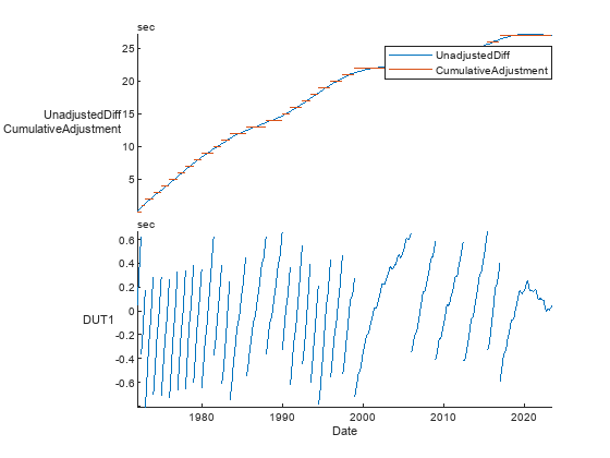
The IERS makes leap second adjustments to keep UTC roughly in sync with UT1. To show how this adjustment works, plot the CumulativeAdjustment state variable as a piecewise-constant step function over time. The step function approximates the accumulated excess LOD, so subtracting it keeps DUT1 small. For visual confirmation, plot DUT1 along the same time axis by using the stackedplot function. Plot UnadjustedDiff and CumulativeAdjustment together along one _y_-axis, with a legend, and plot DUT1 along a second _y_-axis. Because the events in the attached event table were converted to interval events that cover the entire time range, it is redundant to plot events. So, specify the EventsVisible name-value argument as "off".
stackedplot(IERSdata1972,{["UnadjustedDiff","CumulativeAdjustment"],"DUT1"},EventsVisible="off")
Choose Events or State Variables
The two representations, a separate list of events and a state variable defined at all times, are conceptually different. In some cases, there might not be a useful definition of a "state" that corresponds to the periods between instantaneous events. But when there is, the two representations are equivalent and useful in similar ways. For example, to select all the data after the 22nd leap second but before the 23rd, you can use an event filter and timerange.
EF = eventfilter(IERSdata1972)
EF = eventfilter with no constraints and no selected variables
<unconstrained>VariableNames: Date, Type, CumulativeAdjustment, UnadjustedDiff, EventEnds
from22to23 = timerange(EF.CumulativeAdjustment == seconds(22),EF.CumulativeAdjustment == seconds(23),"openright"); data22to23 = IERSdata1972(from22to23,:)
data22to23=2557×4 timetable
Date ExcessLOD UnadjustedDiff CumulativeAdjustment DUT1
___________ _____________ ______________ ____________________ ____________
<1 event> 31-Dec-1998 0.0010954 sec 21.282 sec 22 sec -0.71811 sec
<1 event> 01-Jan-1999 0.0009738 sec 21.283 sec 22 sec -0.71702 sec
<1 event> 02-Jan-1999 0.000888 sec 21.284 sec 22 sec -0.71604 sec
<1 event> 03-Jan-1999 0.0008605 sec 21.285 sec 22 sec -0.71516 sec
<1 event> 04-Jan-1999 0.0008798 sec 21.286 sec 22 sec -0.71429 sec
<1 event> 05-Jan-1999 0.0008935 sec 21.287 sec 22 sec -0.71342 sec
<1 event> 06-Jan-1999 0.0009693 sec 21.287 sec 22 sec -0.71252 sec
<1 event> 07-Jan-1999 0.0010658 sec 21.288 sec 22 sec -0.71155 sec
<1 event> 08-Jan-1999 0.0010857 sec 21.29 sec 22 sec -0.71049 sec
<1 event> 09-Jan-1999 0.0010715 sec 21.291 sec 22 sec -0.7094 sec
<1 event> 10-Jan-1999 0.0010519 sec 21.292 sec 22 sec -0.70833 sec
<1 event> 11-Jan-1999 0.0010021 sec 21.293 sec 22 sec -0.70728 sec
<1 event> 12-Jan-1999 0.0008986 sec 21.294 sec 22 sec -0.70628 sec
<1 event> 13-Jan-1999 0.0007891 sec 21.295 sec 22 sec -0.70538 sec
<1 event> 14-Jan-1999 0.0007236 sec 21.295 sec 22 sec -0.70459 sec
<1 event> 15-Jan-1999 0.0006842 sec 21.296 sec 22 sec -0.70386 sec
⋮
As an alternative, you can create a logical subscript from the state variable that selects the same data.
from22to23 = (IERSdata1972.CumulativeAdjustment == seconds(22)); data22to23 = IERSdata1972(from22to23,:)
data22to23=2556×4 timetable
Date ExcessLOD UnadjustedDiff CumulativeAdjustment DUT1
___________ _____________ ______________ ____________________ ____________
<1 event> 31-Dec-1998 0.0010954 sec 21.282 sec 22 sec -0.71811 sec
<1 event> 01-Jan-1999 0.0009738 sec 21.283 sec 22 sec -0.71702 sec
<1 event> 02-Jan-1999 0.000888 sec 21.284 sec 22 sec -0.71604 sec
<1 event> 03-Jan-1999 0.0008605 sec 21.285 sec 22 sec -0.71516 sec
<1 event> 04-Jan-1999 0.0008798 sec 21.286 sec 22 sec -0.71429 sec
<1 event> 05-Jan-1999 0.0008935 sec 21.287 sec 22 sec -0.71342 sec
<1 event> 06-Jan-1999 0.0009693 sec 21.287 sec 22 sec -0.71252 sec
<1 event> 07-Jan-1999 0.0010658 sec 21.288 sec 22 sec -0.71155 sec
<1 event> 08-Jan-1999 0.0010857 sec 21.29 sec 22 sec -0.71049 sec
<1 event> 09-Jan-1999 0.0010715 sec 21.291 sec 22 sec -0.7094 sec
<1 event> 10-Jan-1999 0.0010519 sec 21.292 sec 22 sec -0.70833 sec
<1 event> 11-Jan-1999 0.0010021 sec 21.293 sec 22 sec -0.70728 sec
<1 event> 12-Jan-1999 0.0008986 sec 21.294 sec 22 sec -0.70628 sec
<1 event> 13-Jan-1999 0.0007891 sec 21.295 sec 22 sec -0.70538 sec
<1 event> 14-Jan-1999 0.0007236 sec 21.295 sec 22 sec -0.70459 sec
<1 event> 15-Jan-1999 0.0006842 sec 21.296 sec 22 sec -0.70386 sec
⋮
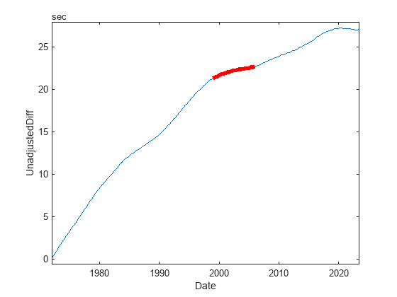
Both representations have their uses. For example, while each event can be plotted as a point, the state variable is the more convenient form for highlighting regions between events in a plot. To highlight the region between the 22nd and 23rd leap second, use the from22to23 logical subscript created from CumulativeAdjustment.
plot(IERSdata1972,"UnadjustedDiff"); hold on plot(IERSdata1972(from22to23,:),"UnadjustedDiff",Color="r",LineWidth=4); hold off
You can switch between the two representations. In this case, to get the leap second event dates from CumulativeAdjustment, find the locations where the adjustment changes, and subtract one day. The eventTimes output represents the dates on which leap seconds were added, which are instantaneous events.
eventTimes = IERSdata1972.Date(diff(IERSdata1972.CumulativeAdjustment) ~= 0) + caldays(1)
eventTimes = 55×1 datetime 29-Jun-1972 30-Jun-1972 30-Dec-1972 31-Dec-1972 30-Dec-1973 31-Dec-1973 30-Dec-1974 31-Dec-1974 30-Dec-1975 31-Dec-1975 30-Dec-1976 31-Dec-1976 30-Dec-1977 31-Dec-1977 30-Dec-1978 31-Dec-1978 30-Dec-1979 31-Dec-1979 29-Jun-1981 30-Jun-1981 29-Jun-1982 30-Jun-1982 29-Jun-1983 30-Jun-1983 29-Jun-1985 30-Jun-1985 30-Dec-1987 31-Dec-1987 30-Dec-1989 31-Dec-1989 ⋮
To represent events, you can use event tables, with either instantaneous events or interval events, or state variables in timetables. The representation you use depends on which one is more convenient and useful for the data analysis that you plan to conduct. You might even switch between representations as you go. All these representations are useful ways to add information about events to your timestamped data in a timetable.
See Also
eventtable | timetable | datetime | seconds | leapseconds | timerange | stackedplot | readtable | table2timetable | cumsum