Find Events in Timetable Using Event Table - MATLAB & Simulink (original) (raw)
To find and label events in a timetable, attach an eventtable to it. An event table is a timetable of events. An event consists of an event time (when something happened), often an event length or event end time (how long it happened), often an event label (what happened), and sometimes additional information about the event. When you attach an event table to a timetable, it enables you to find and label rows in the timetable that occur during events. By associating timetable rows with events, you can more easily analyze and plot the data that they contain.
This example shows how you can define events in data using information that is already within your timetable. In the example, import a timetable of measurements of the Earth's rotation rate from 1962 to the present. The rotation rate varies as a function of time, causing changes in the excess length-of-day to accumulate. When you plot the excess length-of-day as a function of time, the peaks and troughs in the plot represent events in this data set. To analyze these data with event tables, use the extractevents, eventfilter, and syncevents functions. (A related workflow is to add events from an external data source to your timetable. For more information about that workflow, see Add Event Table from External Data to Timetable.)
Import Timetable with Length-of-Day Measurements
By definition, a day is 86,400 seconds long, where the second has a precise definition in the International System of Units (SI). However, the length of a day actually varies due to several physical causes. It varies with the seasons by as much as 30 seconds over and 21 seconds under the SI definition because of the eccentricity of Earth's orbit and the tilt of its axis. Averaging these seasonal effects enables the definition of the mean solar day, which does not vary in length over a year.
Also, there is a very long-term slowing in the rotational speed of the Earth due to tidal interaction with the moon; a smaller, opposite, shorter-term component believed to be due to melting of continental ice sheets; very short-term cycles on the order of decades; and unpredictable fluctuations due to geological events and other causes. Because of those effects, the length of a mean solar day might increase or decrease. In recent decades, it has fluctuated up and down, but has mostly been 1–3 milliseconds longer than 86,400 seconds. That difference is known as the excess Length of Day, or excess LOD.
For this example, create a timetable that contains the excess LOD for every day from January 1, 1962, to the present. The International Earth Rotation and Reference Systems Service (IERS) collects and publishes this data. However, this data needs preprocessing before storing in a MATLAB timetable because the dates are modified Julian dates. To read the IERS data into a table, use the readtable function. Rename the two variables of interest to MJD and ExcessLOD.
file = "https://datacenter.iers.org/data/latestVersion/223_EOP_C04_14.62-NOW.IAU1980223.txt"; IERSdata = readtable(file,"NumHeaderLines",14); IERSdata.Properties.VariableNames([4 8]) = ["MJD","ExcessLOD"];
To store the excess LOD values in a timetable, convert the modified Julian dates to datetime values. Use the datetime function with the "ConvertFrom","mjd" name-value argument. Then convert IERSdata from a table to a timetable using the table2timetable function.
IERSdata.Date = datetime(IERSdata.MJD,"ConvertFrom","mjd"); IERSdata.ExcessLOD = seconds(IERSdata.ExcessLOD); IERSdata = table2timetable(IERSdata(:,["Date","ExcessLOD"]))
IERSdata=22458×1 timetable
Date ExcessLOD
___________ ____________
01-Jan-1962 0.001723 sec
02-Jan-1962 0.001669 sec
03-Jan-1962 0.001582 sec
04-Jan-1962 0.001496 sec
05-Jan-1962 0.001416 sec
06-Jan-1962 0.001382 sec
07-Jan-1962 0.001413 sec
08-Jan-1962 0.001505 sec
09-Jan-1962 0.001628 sec
10-Jan-1962 0.001738 sec
11-Jan-1962 0.001794 sec
12-Jan-1962 0.001774 sec
13-Jan-1962 0.001667 sec
14-Jan-1962 0.00151 sec
15-Jan-1962 0.001312 sec
16-Jan-1962 0.001112 sec
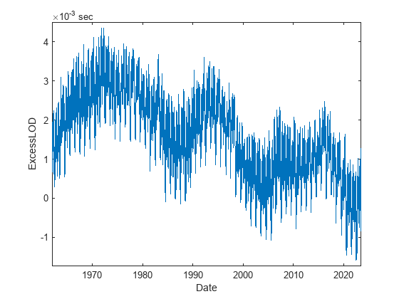
⋮Plot the excess LOD as a function of time. When the input is a timetable, the plot function automatically plots the timetable variables that you specify against the row times.
plot(IERSdata,"ExcessLOD")
Extract Events from Timetable
Since the 1960s there have been several periods when the excess LOD decreased over the short term. If you smooth the excess LOD data, you can see this local behavior more easily.
To smooth the excess LOD, use the smoothdata function. Then plot the smoothed data and the excess LOD using the stackedplot function. It creates a plot of every variable in a timetable and stacks the plots.
IERSdata.SmoothedELOD = smoothdata(seconds(IERSdata.ExcessLOD),"loess","SmoothingFactor",.4); stackedplot(IERSdata)
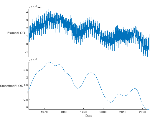
The peaks and troughs of the smoothed data show where the short-term trend changed direction. After reaching a peak, the excess LOD decreases. After reaching a trough, the excess LOD increases. The peaks and troughs are notable events in this data set.
To identify the peaks and troughs in the smoothed data, use the islocalmax and islocalmin functions. Then get the date and the value of the excess LOD for each peak and trough. Create a categorical array with two types, peak and trough, which describe these two types of events.
peaks = find(islocalmax(IERSdata.SmoothedELOD)); troughs = find(islocalmin(IERSdata.SmoothedELOD)); typeLabels = categorical([zeros(size(peaks)); ones(size(troughs))],[0 1],["peak","trough"]);
Store the peaks and troughs in an event table. To extract the times of the peaks and troughs from IERSdata, use the extractevents function. These times are the event times of the event table. The values in typeLabels are the event labels for these events. You can consider the peaks and troughs to be instantaneous events because they occur on specific dates in the timetable.
extremaEvents = extractevents(IERSdata,[peaks;troughs],EventLabels=typeLabels)
extremaEvents = 10×1 eventtable Event Labels Variable: EventLabels Event Lengths Variable:
   Date        EventLabels
___________    ___________

08-Jul-1972      peak
26-Jun-1977      peak
14-Oct-1993      peak
18-Feb-2008      peak
16-Dec-2015      peak
10-Aug-1975      trough
07-Jan-1987      trough
02-Nov-2003      trough
09-Jul-2010      trough
12-Sep-2022      trough
Attach Event Table to Timetable
Attach the new event table to the Events property of IERSdata. To find and label events using an event table, you must first attach it to a timetable. While this timetable has over 22,000 rows, the attached event table identifies nine events that occur within the time spanned by the timetable.
IERSdata.Properties.Events = extremaEvents; IERSdata.Properties
ans = TimetableProperties with properties:
         Description: ''
            UserData: []
      DimensionNames: {'Date'  'Variables'}
       VariableNames: {'ExcessLOD'  'SmoothedELOD'}
VariableDescriptions: {}
       VariableUnits: {}
  VariableContinuity: []
            RowTimes: [22458×1 datetime]
           StartTime: 01-Jan-1962
          SampleRate: NaN
            TimeStep: 1d
              Events: [10×1 eventtable]
    CustomProperties: No custom properties are set.
  Use addprop and rmprop to modify CustomProperties.
Plot Events Against Data
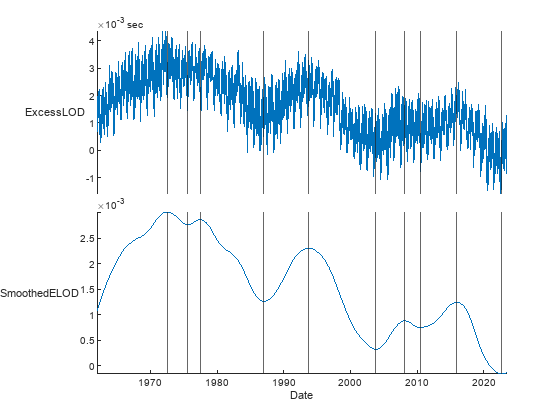
One way to plot the events is to use the stackedplot function. If the input timetable has an attached event table, then stackedplot plots the events on the stacked plot. It plots instantaneous events as vertical lines and interval events as shaded regions.
For example, create a stacked plot of data in IERSdata.
The stackedplot function plots all events using the same style. To plot events using different styles for different kinds of events, use the plot function and specify markers for different events.
For example, make a plot where you mark the peaks using triangles pointed upward and troughs using triangles pointed downward. Start by using the plot function to plot the excess LOD. Then overplot the smoothed excess LOD as a green curve.
plot(IERSdata.Date,IERSdata.ExcessLOD,"b-"); hold on plot(IERSdata.Date,IERSdata.SmoothedELOD,"g-","LineWidth",2); hold off ylabel("Excess LOD");

Next, find the row times that correspond to the peaks and troughs. A convenient way to select the times of these events is to use an eventfilter.
Create an event filter from the event table attached to IERSdata, by using the eventfilter function. You can use the event filter as a row subscript to select rows that occur at events.
EF = eventfilter(IERSdata)
EF = eventfilter with no constraints and no selected variables
<unconstrained>VariableNames: Date, EventLabels
Subscript into IERSdata to show the rows that occur at peaks of the smoothed excess LOD.
IERSdataPeaks = IERSdata(EF.EventLabels == "peak",:)
IERSdataPeaks=5×2 timetable Date ExcessLOD SmoothedELOD ___________ _____________ ____________
peak    08-Jul-1972     0.002262 sec      0.0030098
peak    26-Jun-1977     0.002236 sec      0.0028586
peak    14-Oct-1993    0.0033068 sec      0.0023039
peak    18-Feb-2008     0.000678 sec     0.00087485
peak    16-Dec-2015    0.0016321 sec      0.0012395
Show the rows that occur at troughs of the smoothed excess LOD.
IERSdataTroughs = IERSdata(EF.EventLabels == "trough",:)
IERSdataTroughs=5×2 timetable Date ExcessLOD SmoothedELOD ___________ ______________ ____________
trough    10-Aug-1975      0.002726 sec      0.0027631
trough    07-Jan-1987     0.0016989 sec      0.0012593
trough    02-Nov-2003     0.0001406 sec     0.00031328
trough    09-Jul-2010    -0.0006137 sec     0.00074505
trough    12-Sep-2022     0.0003547 sec    -0.00016658
Plot the peaks using triangles pointed upward and the troughs using triangles pointed downward.
hold on hpeaks = plot(IERSdataPeaks,"SmoothedELOD",LineStyle="none",Marker="^",MarkerFaceColor="y"); htroughs = plot(IERSdataTroughs,"SmoothedELOD",LineStyle="none",Marker="v",MarkerFaceColor="y"); hold off

Create Event Table of Interval Events
From peak to trough, the excess LOD decreases, meaning that the Earth's rotation speeds up during that interval. From trough to peak, the excess LOD increases, meaning that the rotation slows down. You can consider these periods of decreasing and increasing excess LOD to be interval events. These events persist over significant lengths of time within the excess LOD data set.
Change the event table into an event table that stores interval events. First, assign the attached event table to a more convenient local variable. Then sort it by the event times.
intervalEvents = IERSdata.Properties.Events; intervalEvents = sortrows(intervalEvents)
intervalEvents = 10×1 eventtable Event Labels Variable: EventLabels Event Lengths Variable:
   Date        EventLabels
___________    ___________

08-Jul-1972      peak
10-Aug-1975      trough
26-Jun-1977      peak
07-Jan-1987      trough
14-Oct-1993      peak
02-Nov-2003      trough
18-Feb-2008      peak
09-Jul-2010      trough
16-Dec-2015      peak
12-Sep-2022      trough
To turn the events into interval events, assign event end times to them. In this data set, the end of every interval is the day before the start of the next interval. (However, let the "end" of the last interval be the last date in IERSdata.) Assign the event end times as a new variable in intervalEvents. Then assign the new variable to the EventEndsVariable property of the event table. This assignment turns the events into interval events.
endEvents = [intervalEvents.Date(2:end) - 1 ; IERSdata.Date(end)]; intervalEvents.EventEnds = endEvents; intervalEvents.Properties.EventEndsVariable = "EventEnds"
intervalEvents = 10×2 eventtable Event Labels Variable: EventLabels Event Ends Variable: EventEnds
   Date        EventLabels     EventEnds
___________    ___________    ___________

08-Jul-1972      peak         09-Aug-1975
10-Aug-1975      trough       25-Jun-1977
26-Jun-1977      peak         06-Jan-1987
07-Jan-1987      trough       13-Oct-1993
14-Oct-1993      peak         01-Nov-2003
02-Nov-2003      trough       17-Feb-2008
18-Feb-2008      peak         08-Jul-2010
09-Jul-2010      trough       15-Dec-2015
16-Dec-2015      peak         11-Sep-2022
12-Sep-2022      trough       27-Jun-2023
The labels "peaks" and "troughs" were appropriate labels for instantaneous events because they identified inflection points on the smoothed excess LOD curve. But they are not appropriate labels for interval events. Change the labels to "decreasingLOD" and "increasingLOD".
intervalEvents.EventLabels = renamecats(intervalEvents.EventLabels,["decreasingLOD","increasingLOD"])
intervalEvents = 10×2 eventtable Event Labels Variable: EventLabels Event Ends Variable: EventEnds
   Date         EventLabels      EventEnds
___________    _____________    ___________

08-Jul-1972    decreasingLOD    09-Aug-1975
10-Aug-1975    increasingLOD    25-Jun-1977
26-Jun-1977    decreasingLOD    06-Jan-1987
07-Jan-1987    increasingLOD    13-Oct-1993
14-Oct-1993    decreasingLOD    01-Nov-2003
02-Nov-2003    increasingLOD    17-Feb-2008
18-Feb-2008    decreasingLOD    08-Jul-2010
09-Jul-2010    increasingLOD    15-Dec-2015
16-Dec-2015    decreasingLOD    11-Sep-2022
12-Sep-2022    increasingLOD    27-Jun-2023
The first interval starts with the first peak. However, IERSdata has earlier rows leading up to that peak. To add that period as an interval of increasing excess LOD, add another row to the event table. Its event time is the first date in IERSdata. Its event end time is the day before the first peak.
intervalEvents(IERSdata.Date(1),:) = {"increasingLOD",intervalEvents.Date(1) - 1}; intervalEvents = sortrows(intervalEvents)
intervalEvents = 11×2 eventtable Event Labels Variable: EventLabels Event Ends Variable: EventEnds
   Date         EventLabels      EventEnds
___________    _____________    ___________

01-Jan-1962    increasingLOD    07-Jul-1972
08-Jul-1972    decreasingLOD    09-Aug-1975
10-Aug-1975    increasingLOD    25-Jun-1977
26-Jun-1977    decreasingLOD    06-Jan-1987
07-Jan-1987    increasingLOD    13-Oct-1993
14-Oct-1993    decreasingLOD    01-Nov-2003
02-Nov-2003    increasingLOD    17-Feb-2008
18-Feb-2008    decreasingLOD    08-Jul-2010
09-Jul-2010    increasingLOD    15-Dec-2015
16-Dec-2015    decreasingLOD    11-Sep-2022
12-Sep-2022    increasingLOD    27-Jun-2023
You can add more data that describes these events in additional event table variables. For example, compute the average change in excess LOD during each interval (in units of seconds of daily excess LOD per year). Add that information to the interval events as a new variable.
dTime = intervalEvents.EventEnds - intervalEvents.Date; dExcess = IERSdata.SmoothedELOD(intervalEvents.EventEnds) - IERSdata.SmoothedELOD(intervalEvents.Date); intervalEvents.AnnualAvgChange = seconds(dExcess ./ years(dTime))
intervalEvents = 11×3 eventtable Event Labels Variable: EventLabels Event Ends Variable: EventEnds
   Date         EventLabels      EventEnds     AnnualAvgChange
___________    _____________    ___________    _______________

01-Jan-1962    increasingLOD    07-Jul-1972     0.00018435 sec
08-Jul-1972    decreasingLOD    09-Aug-1975    -7.9965e-05 sec
10-Aug-1975    increasingLOD    25-Jun-1977     5.0921e-05 sec
26-Jun-1977    decreasingLOD    06-Jan-1987     -0.0001678 sec
07-Jan-1987    increasingLOD    13-Oct-1993     0.00015441 sec
14-Oct-1993    decreasingLOD    01-Nov-2003    -0.00019811 sec
02-Nov-2003    increasingLOD    17-Feb-2008     0.00013081 sec
18-Feb-2008    decreasingLOD    08-Jul-2010    -5.4428e-05 sec
09-Jul-2010    increasingLOD    15-Dec-2015     9.0984e-05 sec
16-Dec-2015    decreasingLOD    11-Sep-2022    -0.00020868 sec
12-Sep-2022    increasingLOD    27-Jun-2023     4.5288e-05 sec
These results show that the mean solar day, averaged over an entire year, has been decreasing over the last few years by about 0.3 milliseconds per year. The mean solar day is currently near or even slightly less than 86,400 seconds. However, many experts believe that this trend will not continue.
Create Stacked Plot of Interval Events
Create a simple stacked plot of the intervals when the excess LOD was increasing. First, create a subtable of intervalEvents with increasing excess LOD.
increasingEvents = intervalEvents(intervalEvents.EventLabels == "increasingLOD",:)
increasingEvents = 6×3 eventtable Event Labels Variable: EventLabels Event Ends Variable: EventEnds
Date EventLabels EventEnds AnnualAvgChange
___________ _____________ ___________ _______________
01-Jan-1962 increasingLOD 07-Jul-1972 0.00018435 sec
10-Aug-1975 increasingLOD 25-Jun-1977 5.0921e-05 sec
07-Jan-1987 increasingLOD 13-Oct-1993 0.00015441 sec
02-Nov-2003 increasingLOD 17-Feb-2008 0.00013081 sec
09-Jul-2010 increasingLOD 15-Dec-2015 9.0984e-05 sec
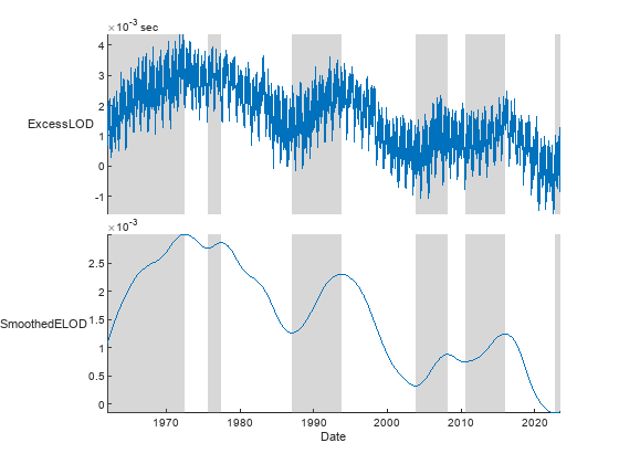
12-Sep-2022 increasingLOD 27-Jun-2023 4.5288e-05 sec Attach increasingEvents to the Events property of IERSdata. Then make a stacked plot that shows only the intervals with increasing excess LOD as shaded regions.
IERSdata.Properties.Events = increasingEvents; stackedplot(IERSdata)
Convert Interval Events to State Variable
To work with intervals of decreasing and increasing excess LOD, attach intervalEvents to the Events property of IERSdata. You can convert the interval events to a state variable, and make more complex plots of the events associated with these data.
IERSdata.Properties.Events = intervalEvents;
The event table records interval events during which the smoothed excess LOD reached a peak and began a decrease or reached a trough and began an increase. Another way to represent those changes is as a state variable within the timetable itself. To copy event data from an attached event table to variables of the main timetable, use the syncevents function. As a result of this call, IERSdata has new variables, EventLabels and AnnualAvgChange, copied from the attached event table.
IERSdata = syncevents(IERSdata)
IERSdata=22458×4 timetable Date ExcessLOD SmoothedELOD EventLabels AnnualAvgChange ___________ ____________ ____________ _____________ _______________
increasingLOD 01-Jan-1962 0.001723 sec 0.0010716 increasingLOD 0.00018435 sec
increasingLOD 02-Jan-1962 0.001669 sec 0.0010728 increasingLOD 0.00018435 sec
increasingLOD 03-Jan-1962 0.001582 sec 0.0010739 increasingLOD 0.00018435 sec
increasingLOD 04-Jan-1962 0.001496 sec 0.0010751 increasingLOD 0.00018435 sec
increasingLOD 05-Jan-1962 0.001416 sec 0.0010762 increasingLOD 0.00018435 sec
increasingLOD 06-Jan-1962 0.001382 sec 0.0010773 increasingLOD 0.00018435 sec
increasingLOD 07-Jan-1962 0.001413 sec 0.0010785 increasingLOD 0.00018435 sec
increasingLOD 08-Jan-1962 0.001505 sec 0.0010796 increasingLOD 0.00018435 sec
increasingLOD 09-Jan-1962 0.001628 sec 0.0010807 increasingLOD 0.00018435 sec
increasingLOD 10-Jan-1962 0.001738 sec 0.0010818 increasingLOD 0.00018435 sec
increasingLOD 11-Jan-1962 0.001794 sec 0.001083 increasingLOD 0.00018435 sec
increasingLOD 12-Jan-1962 0.001774 sec 0.0010841 increasingLOD 0.00018435 sec
increasingLOD 13-Jan-1962 0.001667 sec 0.0010852 increasingLOD 0.00018435 sec
increasingLOD 14-Jan-1962 0.00151 sec 0.0010864 increasingLOD 0.00018435 sec
increasingLOD 15-Jan-1962 0.001312 sec 0.0010875 increasingLOD 0.00018435 sec
increasingLOD 16-Jan-1962 0.001112 sec 0.0010886 increasingLOD 0.00018435 sec
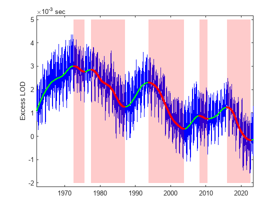
⋮Next, highlight the segments in the plot where excess LOD is increasing in green and decreasing in red. In this case, it is more convenient to use the EventLabels state variable in IERSdata because you need to change the color at every data point in each segment.
plot(IERSdata.Date,IERSdata.ExcessLOD,"b-"); hold on plot(IERSdata.Date,IERSdata.SmoothedELOD,"g-","LineWidth",2); ylabel("Excess LOD"); decreasing = (IERSdata.EventLabels == "decreasingLOD"); plot(IERSdata.Date(decreasing),IERSdata.SmoothedELOD(decreasing),'r.'); hold off

Alternatively, highlight the background in regions of decreasing excess LOD. In this case, it is more convenient to use the interval events from the attached event table, because you only need the start and end times of the intervals when excess LOD decreases.
hold on decreasingEvents = IERSdata.Properties.Events; decreasingEvents = decreasingEvents(decreasingEvents.EventLabels == "decreasingLOD",:); startEndTimes = [decreasingEvents.Date decreasingEvents.EventEnds]; h = fill(startEndTimes(:,[1 2 2 1]),[-.002 -.002 .005 .005],"red","FaceAlpha",.2,"LineStyle","none"); hold off
Find More Complex Events in Data
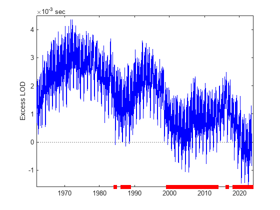
The excess LOD has both increased and decreased since the 1960s. Indeed, in many years there were short periods when the raw excess LOD was significantly negative. These are only very short-term fluctuations, but during those periods the Earth was rotating one millisecond or more faster than 86,400 SI seconds.
plot(IERSdata.Date,IERSdata.ExcessLOD,"b-"); ylabel("Excess LOD"); hold on line(IERSdata.Date([1 end]),[0 0],"Color","k","LineStyle",":") hold off ylabel("Excess LOD");

Identify the dates on which the excess LOD was negative. Extract those dates and the excess LODs into an event table. As there are over 1400 rows, display the first few rows of the event table.
negLOD = extractevents(IERSdata,IERSdata.ExcessLOD < 0,EventDataVariables="ExcessLOD"); negLODhead = head(negLOD,5)
negLODhead = 5×1 eventtable Event Labels Variable: Event Lengths Variable:
   Date          ExcessLOD
___________    _____________

12-Jul-1984    -2.27e-05 sec
13-Jul-1984    -9.38e-05 sec
14-Jul-1984     -3.8e-06 sec
09-Jun-1986     -5.5e-06 sec
02-Aug-1986    -1.33e-05 sec
Identify the years in which those days of excess LOD occurred. Then use the retime function to find the minimum excess LOD in each of those years and return a new event table. (Because an event table is a kind of timetable, you can call timetable functions on event tables.) These are interval events in one sense but are stored as instantaneous events marked only by their year.
negYears = unique(dateshift(negLOD.Date,"start","year")); negYears.Format = "uuuu"; negLODEvents = retime(negLOD,negYears,"min"); negLODEvents.Properties.VariableNames = "MinExcessLOD"
negLODEvents = 26×1 eventtable Event Labels Variable: Event Lengths Variable:
Date     MinExcessLOD
____    ______________

1984     -9.38e-05 sec
1986     -1.33e-05 sec
1987    -0.0001492 sec
1988     -7.06e-05 sec
1999    -0.0001063 sec
2000     -0.000311 sec
2001    -0.0007064 sec
2002    -0.0007436 sec
2003    -0.0009769 sec
2004    -0.0010672 sec
2005    -0.0010809 sec
2006    -0.0003865 sec
2007    -0.0006192 sec
2008    -0.0003945 sec
2009    -0.0004417 sec
2010     -0.000784 sec
2011     -0.000342 sec
2012    -0.0003178 sec
2013    -0.0003593 sec
2016     -1.95e-05 sec
2018    -0.0006457 sec
2019    -0.0009571 sec
2020    -0.0014663 sec
2021     -0.001452 sec
2022    -0.0015903 sec
2023           NaN sec
In the plot of excess LOD, mark the time axis red for each year that had periods when the excess LOD was negative. In this data set, such years happen more frequently after the year 2000.
hold on plot([negLODEvents.Date negLODEvents.Date+calyears(1)],[-.0016 -.0016],"r-","lineWidth",6); ylim(seconds([-.0016 .0045])); hold off
To represent events, you can use event tables, with either instantaneous events or interval events, or state variables in timetables. The representation you use depends on which one is more convenient and useful for the data analysis that you plan to conduct. You might even switch between representations as you go. All these representations are useful ways to add information about events to your timestamped data in a timetable.
See Also
eventtable | timetable | datetime | retime | smoothdata | islocalmax | islocalmin | seconds | timerange | stackedplot | readtable | table2timetable