exportgraphics - Save plot or graphics content to file - MATLAB (original) (raw)
Save plot or graphics content to file
Since R2020a
Syntax
Description
exportgraphics([obj](#mw%5F0f2a4f3a-4308-4733-a4ce-30925773dd4b),[filename](#mw%5F3db70293-26d3-4e3f-9abf-6b96488e4dde)) saves the contents of the graphics object specified by obj to a file. The graphics object can be any type of axes, a figure, a standalone visualization, a tiled chart layout, or a container within the figure. The resulting graphic is tightly cropped to a thin margin surrounding your content.
exportgraphics([obj](#mw%5F0f2a4f3a-4308-4733-a4ce-30925773dd4b),[filename](#mw%5F3db70293-26d3-4e3f-9abf-6b96488e4dde),[Name,Value](#namevaluepairarguments)) specifies additional options for saving the file. For example,exportgraphics(gca,"myplot.jpg","Resolution",300) saves the contents of the current axes as a 300-DPI image file.
Examples
Export Axes as Image File
Create a line plot and get the current axes. Then save the contents of the axes as a JPEG file.
plot(rand(5,5)) ax = gca; exportgraphics(ax,'LinePlot.jpg')

Specify Image Resolution
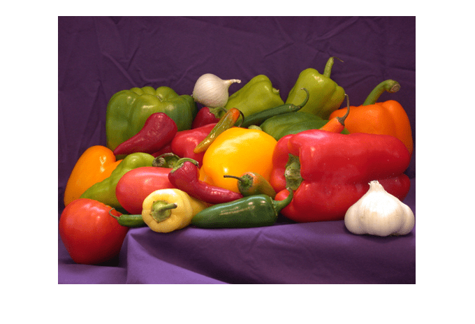
Display an image and get the current axes. Then save the contents of the axes as a 300-DPI JPEG file.
I = imread('peppers.png'); imshow(I) ax = gca; exportgraphics(ax,'Peppers300.jpg','Resolution',300)
Export Figure
Display a plot with an annotation that extends beyond the bounds of the axes. Save the contents of the figure as a PDF file.
plot(1:10) annotation('textarrow',[0.06 0.5],[0.73 0.5],'String','y = x ') f = gcf; exportgraphics(f,'AnnotatedPlot.pdf')

Export as PDF Containing Only Vector Graphics
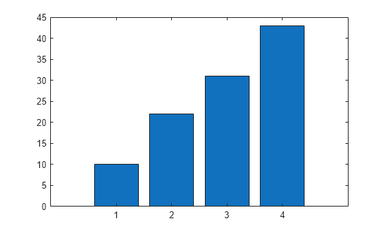
Display a bar chart and get the current axes. Then save the contents of the axes as a PDF containing only vector graphics.
bar([10 22 31 43]) ax = gca; exportgraphics(ax,'BarChart.pdf','ContentType','vector')
Export Multipage PDF
To create multipage PDFs, set the 'Append' name-value argument to true.
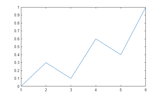
For example, create a line plot and save the contents of the axes to the file myplots.pdf.
plot([0 0.3 0.1 0.6 0.4 1]) ax = gca; exportgraphics(ax,'myplots.pdf')
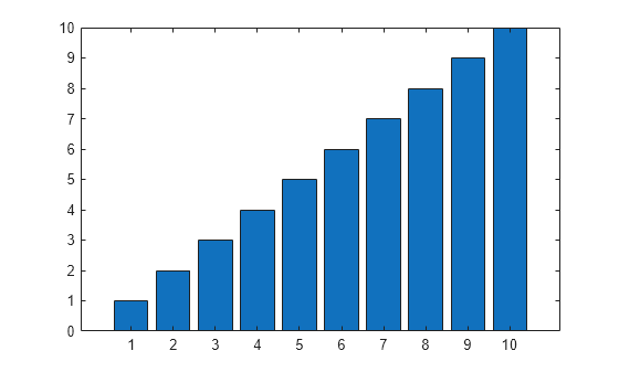
Next, create a bar chart and save the contents of the axes as a second page in myplots.pdf.
bar(1:10) exportgraphics(ax,'myplots.pdf','Append',true)
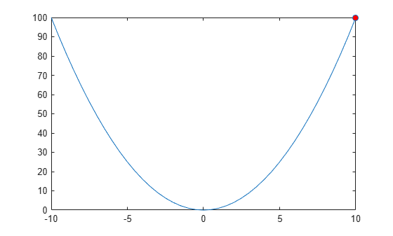
Export Animated GIF
Plot a parabola with one marker. Change the location of the marker with every iteration of a for loop, and capture the changes as frames in an animated GIF.
x = -10:0.5:10; y = x.^2; p = plot(x,y,"-o","MarkerFaceColor","red"); for i=1:41 p.MarkerIndices = i; exportgraphics(gca,"parabola.gif","Append",true) end
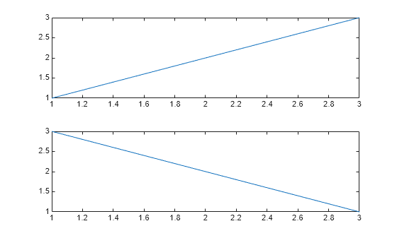
Export Tiled Chart Layout
Display two plots in a tiled chart layout. Then save both plots as a PDF by passing the TiledChartLayout object to the exportgraphics function.
t = tiledlayout(2,1); nexttile plot([1 2 3]) nexttile plot([3 2 1]) exportgraphics(t,'Layout.pdf')
If you want to save just one of the plots in the layout, call the nexttile function with the axes return argument. Then pass the axes to the exportgraphics function.
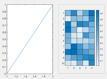
Export Heatmap as PDF With Transparent Background
Display a heatmap chart. Then save the chart as a PDF containing only vector graphics with a transparent background.
h = heatmap(rand(10,10)); exportgraphics(h,'Hmap.pdf','BackgroundColor','none','ContentType','vector')

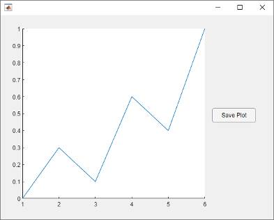
Create App for Saving Plot
Create a program file called saveapp.m that displays a plot and a button for saving the axes content. In the callback function for the button, call theuiputfile function to prompt the user for a file name and location. Then call the exportgraphics function with the full path to the specified file.
function saveapp f = uifigure; ax = uiaxes(f,"Position",[25 25 400 375]); plot(ax,[0 0.3 0.1 0.6 0.4 1]) b = uibutton(f,"Position",[435 200 90 30],"Text","Save Plot"); b.ButtonPushedFcn = @buttoncallback;
function buttoncallback(~,~)
    filter = {"*.jpg";"*.png";"*.tif";"*.pdf";"*.eps"};
    [filename,filepath] = uiputfile(filter);
    if ischar(filename)
        exportgraphics(ax,[filepath filename]);
    end
end
end
Run the app by calling the saveapp function. When you click theSave Plot button in the app, a dialog box prompts you for a file name and location. Then the axes content is saved in the specified file. The area surrounding the axes, including the button, is not included in the file.
Input Arguments
obj — Graphics object
axes | figure | standalone visualization | tiled chart layout | ...
Graphics object, specified as one of these objects:
- Any type of axes: an
Axes,PolarAxes, orGeographicAxesobject. - A figure created with either the figure or uifigure function.
- A standalone visualization such as a heatmap chart.
- A tiled chart layout, which you create with the tiledlayout function.
- A container within a figure: a
Panel,Tab, orButtonGroupobject.
Capture Area
exportgraphics captures the contents of the object you specify. It does not capture UI components such as buttons or sliders.
It also does not capture adjacent containers or child containers. For example, consider a figure containing a line plot with an adjacent panel containing a heatmap:
f = figure; ax = axes(f,"Position",[0.1 0.1 0.4 0.8]); plot(ax,[0 1]) p = uipanel(f,"Position",[0.55 0.1 0.4 0.8]); heatmap(p,rand(10,5))
exportgraphics(f,"myfigure.png") exportgraphics(p,"mypanel.png")
When you run the preceding code, myfigure.png contains the line plot, but not the heatmap. Similarly, mypanel.png contains the heatmap, but not the line plot.
filename — File name
character vector | string scalar
File name, specified as a character vector or a string scalar that includes the file extension. If filename does not include a full path, MATLAB® saves the file in the current folder. You must have permission to write to the file.
The following table lists the supported file formats and the file extensions (which are not case sensitive).
| File Format | File Extension |
|---|---|
| Joint Photographic Experts Group (JPEG) | "jpg" or "jpeg" |
| Portable Network Graphics (PNG) | "png" |
| Tagged Image File Format (TIFF) | "tif" or "tiff" |
| Graphics Interchange Format (GIF) | "gif" |
| Portable Document Format (PDF)The PDF includes embeddable fonts when the ContentType is set to"vector". | "pdf" |
| Enhanced Metafile for Windows® systems only (EMF) | "emf" |
| Encapsulated PostScript® (EPS) | "eps" |
Example: exportgraphics(gca,"myfile.jpg") saves the contents of the current axes to a JPEG file called myfile.jpg.
Name-Value Arguments
Specify optional pairs of arguments asName1=Value1,...,NameN=ValueN, where Name is the argument name and Value is the corresponding value. Name-value arguments must appear after other arguments, but the order of the pairs does not matter.
Before R2021a, use commas to separate each name and value, and enclose Name in quotes.
Example: exportgraphics(gca,"myplot.jpg","Resolution",300) saves the contents of the current axes to a 300-DPI image file.
ContentType — Type of content
"auto" (default) | "vector" | "image"
Type of content to store when saving as an EMF, EPS, or PDF file. Specify the value as one of these options:
"auto"— MATLAB controls whether the content is a vector graphic or an image."vector"— Stores the content as a vector graphic that can scale to any size. If you are saving a PDF file, embeddable fonts are included in the file."image"— Rasterizes the content into one or more images within the file.
Note
- The
"vector"option is not supported for JPEG, TIFF, PNG, and GIF files. - If you specify the
"vector"option, some visualizations might contain stray lines or other artifacts.
Resolution — Resolution (DPI)
150 (default) | whole number
Resolution in dots per inch (DPI), specified as a whole number that is greater than or equal to 1.
Specifying the resolution has no effect when the ContentType is "vector".
Data Types: single | double | int8 | int16 | int32 | int64 | uint8 | uint16 | uint32 | uint64
BackgroundColor — Background color
[1 1 1] (default) | "current" | "none" | RGB triplet | "r" | "g" | "b" | ...
Background color, specified as "current","none", an RGB triplet, a hexadecimal color code, or a color name. The background color controls the color of the margin that surrounds the axes or chart.
- A value of
"current"sets the background color to the parent container's color. - A value of
"none"sets the background color to transparent or white, depending on the file format and the value ofContentType:- Transparent — For files with
ContentType="vector" - White — For image files, or when
ContentType="image" - When
ContentType="auto", MATLAB sets the background color according to the heuristic it uses to determine the type content to save.
- Transparent — For files with
- Alternatively, specify a custom color or a named color.
Custom Colors and Named Colors
RGB triplets and hexadecimal color codes are useful for specifying custom colors.
- An RGB triplet is a three-element row vector whose elements specify the intensities of the red, green, and blue components of the color. The intensities must be in the range
[0,1]; for example,[0.4 0.6 0.7]. - A hexadecimal color code is a character vector or a string scalar that starts with a hash symbol (
#) followed by three or six hexadecimal digits, which can range from0toF. The values are not case sensitive. Thus, the color codes"#FF8800","#ff8800","#F80", and"#f80"are equivalent.
Alternatively, you can specify some common colors by name. This table lists the named color options, the equivalent RGB triplets, and hexadecimal color codes.
| Color Name | Short Name | RGB Triplet | Hexadecimal Color Code | Appearance |
|---|---|---|---|---|
| "red" | "r" | [1 0 0] | "#FF0000" |  |
| "green" | "g" | [0 1 0] | "#00FF00" |  |
| "blue" | "b" | [0 0 1] | "#0000FF" |  |
| "cyan" | "c" | [0 1 1] | "#00FFFF" |  |
| "magenta" | "m" | [1 0 1] | "#FF00FF" |  |
| "yellow" | "y" | [1 1 0] | "#FFFF00" |  |
| "black" | "k" | [0 0 0] | "#000000" |  |
| "white" | "w" | [1 1 1] | "#FFFFFF" |  |
Here are the RGB triplets and hexadecimal color codes for the default colors MATLAB uses in many types of plots.
| RGB Triplet | Hexadecimal Color Code | Appearance |
|---|---|---|
| [0 0.4470 0.7410] | "#0072BD" | ![Sample of RGB triplet [0 0.4470 0.7410], which appears as dark blue](https://www.mathworks.com/help/matlab/ref/colororder1.png) |
| [0.8500 0.3250 0.0980] | "#D95319" | ![Sample of RGB triplet [0.8500 0.3250 0.0980], which appears as dark orange](https://www.mathworks.com/help/matlab/ref/colororder2.png) |
| [0.9290 0.6940 0.1250] | "#EDB120" | ![Sample of RGB triplet [0.9290 0.6940 0.1250], which appears as dark yellow](https://www.mathworks.com/help/matlab/ref/colororder3.png) |
| [0.4940 0.1840 0.5560] | "#7E2F8E" | ![Sample of RGB triplet [0.4940 0.1840 0.5560], which appears as dark purple](https://www.mathworks.com/help/matlab/ref/colororder4.png) |
| [0.4660 0.6740 0.1880] | "#77AC30" | ![Sample of RGB triplet [0.4660 0.6740 0.1880], which appears as medium green](https://www.mathworks.com/help/matlab/ref/colororder5.png) |
| [0.3010 0.7450 0.9330] | "#4DBEEE" | ![Sample of RGB triplet [0.3010 0.7450 0.9330], which appears as light blue](https://www.mathworks.com/help/matlab/ref/colororder6.png) |
| [0.6350 0.0780 0.1840] | "#A2142F" | ![Sample of RGB triplet [0.6350 0.0780 0.1840], which appears as dark red](https://www.mathworks.com/help/matlab/ref/colororder7.png) |
Append — Append content to existing file
false (default) | true
Append content to existing file, specified as true orfalse.
This option is useful for:
- Exporting the content as the last page of an existing PDF file. Call
exportgraphicswith theAppendoption multiple times to add multiple pages. - Exporting the content as the last frame in an animated GIF file. Call
exportgraphicswith theAppendoption multiple times to add multiple frames.
Note
You can use the Append argument to create basic animated GIF files from charts that have the same axes limits. If the axes limits differ between charts, consider using axis("manual") or the xlim, ylim, or zlim functions to freeze the axes limits when creating your charts.
To create animations of images or more elaborate graphics, use imwrite. For more information on using imwrite, see Write Animated GIF.
If you set the Append option to false with the name of an existing file, MATLAB overwrites the contents of the file with the new content.
This option supports PDF and GIF files only.
Colorspace — Color space
"rgb" (default) | "gray" | "cmyk"
Color space of the saved graphic, specified as "rgb","gray", or "cmyk".
"rgb"— Export truecolor RGB content."gray"— Convert the content to grayscale."cmyk"— Convert the content to cyan, magenta, yellow, and black (CMYK). This color space is only supported for EPS files.
Width — Width of saved graphic
"auto" (default) | positive number
Supported in MATLAB Online™ only (since R2024a)
Width of the saved graphic, specified as "auto" or a positive number. To specify a custom width, specify a number. By default, the units are pixels for image files and points for vector graphics files. You can specify different units by using the Units name-value argument. All width values include any padding around the perimeter of the graphic. The saved graphic contains a small margin of padding by default, but you can change it by specifying thePadding name-value argument.
Set Width to "auto" to letexportgraphics select an appropriate width depending on thePreserveAspectRatio value:
- If the
PreserveAspectRatiovalue is"on"(the default value), thenexportgraphicsselects a width that preserves the original aspect ratio according to the specified Height value. - If the
PreserveAspectRatiovalue is"off", thenexportgraphicsuses the default width to save the graphic. The saved graphic might have a different aspect ratio than the original graphic.
Note
When you save image files, the default Width ("auto") depends on the Resolution name-value argument, which is 150 by default. To use the default width and match the on-screen size more closely, specify theResolution name-value argument as the value returned byget(groot,"ScreenPixelsPerInch"). For example:
sppi = get(groot,"ScreenPixelsPerInch"); exportgraphics(gca,"myplot.png","Resolution",sppi)
Height — Height of saved graphic
"auto" (default) | positive number
Supported in MATLAB Online only (since R2024a)
Height of the saved graphic, specified as "auto" or a positive number. To specify a custom height, specify a number. By default, the units are pixels for image files and points for vector graphics files. You can specify different units by using the Units name-value argument. All height values include any padding around the perimeter of the graphic. The saved graphic contains a small margin of padding by default, but you can change it by specifying thePadding name-value argument.
Set Height to "auto" to letexportgraphics select an appropriate height depending on thePreserveAspectRatio value:
- If the
PreserveAspectRatiovalue is"on"(the default value), thenexportgraphicsselects a height that preserves the original aspect ratio according to the specified Width value. - If the
PreserveAspectRatiovalue is"off", thenexportgraphicsuses the default height to save the graphic. The saved graphic might have a different aspect ratio than the original graphic.
Note
When you save image files, the default Height ("auto") depends on the Resolution name-value argument, which is 150 by default. To use the default height and match the on-screen size more closely, specify theResolution name-value argument to the value returned byget(groot,"ScreenPixelsPerInch"). For example:
sppi = get(groot,"ScreenPixelsPerInch"); exportgraphics(gca,"myplot.png","Resolution",sppi)
Padding — Padding around saved graphic
"tight" (default) | "figure" | positive number
Supported in MATLAB Online only (since R2024a)
Padding around the saved graphic, specified as one of the values in this table.
| Value | Description | Example |
|---|---|---|
| "tight" | Include enough padding to include _x_- and_y_-axes labels, a title, and decorations such as legends and colorbars. | Create a bar chart and export it as an image with"tight" padding. Because "tight" is the default padding value, you do not need to specify it.The gray border around the image outlines the captured region. The border is not part of the saved image.bar(1:5) title("My Bar Chart") ax = gca; exportgraphics(ax,"tightpadding.png") 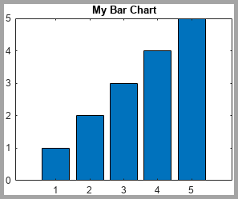 |
| "figure" | Include the same relative amount of padding as shown in the figure window. | Create a bar chart and export it as an image with"figure" padding.The gray border around the image outlines the captured region.bar(1:5) title("My Bar Chart") ax = gca; exportgraphics(ax,"figurepadding.png","Padding","figure")  |
| Positive number | Include the specified amount of padding. By default, the units are pixels for image files and points for vector graphics files. You can specify different units by using the Units name-value argument. | Create a bar chart and export it as an image with 100 pixels of padding. The gray border around the image outlines the captured region.bar(1:5) title("My Bar Chart") ax = gca; exportgraphics(ax,"100pixelpadding.png","Padding",100) 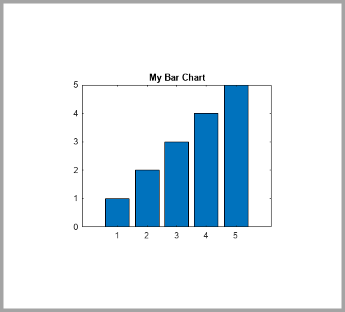 |
Units — Units for width, height, and padding
"auto" (default) | "pixels" | "inches" | "centimeters" | "points"
Supported in MATLAB Online only (since R2024a)
Units for the Width, Height, andPadding values, specified as "auto","pixels" (for images only), "inches","centimeters", or "points" (where 1 point = 1/72 inch).
The default value of "auto" sets the units to"pixels" for image files and "points" for vector graphics files.
PreserveAspectRatio — Preserve original aspect ratio
"auto" (default) | "on" | "off"
Supported in MATLAB Online only (since R2024a)
Preserve original aspect ratio, specified as "auto","on", or "off".
A value of "auto" enables exportgraphics to choose either "on" or "off", depending on whether you specify the Width and Height name-value arguments and whether the combination changes the aspect ratio.exportgraphics preserves the original aspect ratio if you specify the Width or Height name-value argument (but not both). It does not preserve the original aspect ratio if you specify values for both dimensions and those values change aspect ratio.
This table summarizes the behavior of the "on" and"off" values.
| Value | Description | Example |
|---|---|---|
| "on" | Preserve the aspect ratio of the original graphic. If you specify the Width orHeight value (but not both), thenexportgraphics scales the unspecified dimension to preserve the original aspect ratio.If you specify the Width andHeight values, and that combination changes the aspect ratio, exportgraphics adds padding to preserve the original aspect ratio. | Create a bar chart. Then save the chart as an image. Specify only the Width value. exportgraphics scales the height to maintain the original aspect ratio.The gray border around the image outlines the captured region. The border is not part of the saved image.bar(1:5) ax = gca; exportgraphics(ax,"scaledchart.png","Width",250, ... "PreserveAspectRatio","on") 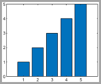 Save the chart as an image with Width andHeight values that result in an image with a different aspect ratio than the original chart.exportgraphics adds padding to achieve the specified dimensions while preserving the aspect ratio of the chart.exportgraphics(ax,"paddedchart.png","Width",250,... "Height",350,"PreserveAspectRatio","on") Save the chart as an image with Width andHeight values that result in an image with a different aspect ratio than the original chart.exportgraphics adds padding to achieve the specified dimensions while preserving the aspect ratio of the chart.exportgraphics(ax,"paddedchart.png","Width",250,... "Height",350,"PreserveAspectRatio","on") 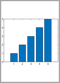 |
| "off" | Do not preserve the original aspect ratio. If theWidth, Height, or both values change the aspect ratio, exportgraphics does not apply any scaling or padding, and the resulting output looks stretched or compressed compared to the original graphic. | Create a bar chart. Then save the chart as an image withWidth and Height values that result in an image with a different aspect ratio than the original chart.The image shows a stretched version of the chart. The gray border around the image outlines the captured region.bar(1:5) ax = gca; exportgraphics(ax,"stretched-chart.png","Width",250,... "Height",350,"PreserveAspectRatio","off") 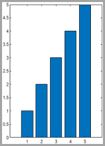 |
Alternative Functionality
Hovering over the Export button ![]() in the axes toolbar reveals a drop-down menu with options for exporting content:
in the axes toolbar reveals a drop-down menu with options for exporting content:
 : Save the content as a tightly cropped image or PDF.
 : Copy the content as an image.
 : Copy the content as a vector graphic.
Version History
Introduced in R2020a
R2024a: Specify dimensions and padding in MATLAB Online
In MATLAB Online, you can specify the width, height, padding, and whether to preserve the aspect ratio of the original graphic.
Use these name-value arguments to control these aspects of the content:
WidthandHeight— Specify the width and height of the output.Padding— Specify the amount of padding around the perimeter of the graphic.Units— Specify the units for the width, height, and padding values.PreserveAspectRatio— Specify whether to automatically add padding to preserve the original aspect ratio if theWidthandHeightvalues conflict with the original aspect ratio of the graphic.
R2022a: Create animated GIF files
Create animated GIF files by calling exportgraphics multiple times with the Append name-value argument set totrue.