graph - Graph with undirected edges - MATLAB (original) (raw)
Graph with undirected edges
Description
graph objects represent undirected graphs, which have direction-less edges connecting the nodes. After you create a graph object, you can learn more about the graph by using object functions to perform queries against the object. For example, you can add or remove nodes or edges, determine the shortest path between two nodes, or locate a specific node or edge.
G = graph([1 1], [2 3]); e = G.Edges G = addedge(G,2,3) G = addnode(G,4) plot(G)
Creation
Syntax
Description
`G` = graph creates an empty undirected graph object, G, which has no nodes or edges.
`G` = graph([A](#bun70n7-A)) creates a graph using a square, symmetric adjacency matrix,A.
- For logical adjacency matrices, the graph has no edge weights.
- For nonlogical adjacency matrices, the graph has edge weights. The location of each nonzero entry in
Aspecifies an edge for the graph, and the weight of the edge is equal to the value of the entry. For example, ifA(2,1) = 10, thenGcontains an edge between node 2 and node 1 with a weight of 10.
`G` = graph([A](#bun70n7-A),[nodenames](#bun70n7-nodenames)) additionally specifies node names. The number of elements innodenames must be equal tosize(A,1).
`G` = graph([A](#bun70n7-A),[NodeTable](#bun70n7-NodeTable)) specifies node names (and possibly other node attributes) using a table,NodeTable. The table must have the same number of rows as A. Specify node names using the table variableName.
`G` = graph([A](#bun70n7-A),___,[type](#bun70n7-type)) specifies a triangle of the adjacency matrix to use in constructing the graph. You must specify A and optionally can specifynodenames or NodeTable. To use only the upper or lower triangle of A to construct the graph, type can be either 'upper' or'lower'.
`G` = graph([A](#bun70n7-A),___,'omitselfloops') ignores the diagonal elements of A and returns a graph without any self-loops. You can use any of the input argument combinations in previous syntaxes.
`G` = graph([s,t](#bun70n7-st)) specifies graph edges (s,t) in node pairs.s and t can specify node indices or node names. graph sorts the edges inG first by source node, and then by target node. If you have edge properties that are in the same order as s and t, use the syntax G = graph(s,t,EdgeTable) to pass in the edge properties so that they are sorted in the same manner in the resulting graph.
`G` = graph([s,t](#bun70n7-st),[weights](#bun70n7-weights)) also specifies edge weights with the arrayweights.
`G` = graph([s,t](#bun70n7-st),[weights](#bun70n7-weights),[nodenames](#bun70n7-nodenames)) specifies node names using the cell array of character vectors or string array, nodenames. s andt cannot contain node names that are not innodenames.
`G` = graph([s,t](#bun70n7-st),[weights](#bun70n7-weights),[NodeTable](#bun70n7-NodeTable)) specifies node names (and possibly other node attributes) using a table,NodeTable. Specify node names using theName table variable. s andt cannot contain node names that are not inNodeTable.
`G` = graph([s,t](#bun70n7-st),[weights](#bun70n7-weights),[num](#bun70n7-num)) specifies the number of nodes in the graph with the numeric scalarnum.
`G` = graph([s,t](#bun70n7-st),___,'omitselfloops') does not add any self-loops to the graph. That is, any k that satisfies s(k) == t(k) is ignored. You can use any of the input argument combinations in previous syntaxes.
`G` = graph([s,t](#bun70n7-st),[EdgeTable](#bun70n7-EdgeTable),___) uses a table to specify edge attributes instead of specifyingweights. The EdgeTable input must be a table with a row for each corresponding pair of elements ins and t. Specify edge weights using the table variable Weight.
`G` = graph([EdgeTable](#bun70n7-EdgeTable)) uses the table EdgeTable to define the graph. With this syntax, the first variable in EdgeTable must be namedEndNodes, and it must be a two-column array defining the edge list of the graph.
`G` = graph([EdgeTable](#bun70n7-EdgeTable),[NodeTable](#bun70n7-NodeTable)) additionally specifies the names (and possibly other attributes) of the graph nodes using a table, NodeTable.
`G` = graph([EdgeTable](#bun70n7-EdgeTable),___,'omitselfloops') does not add self-loops to the graph. That is, any k that satisfies EdgeTable.EndNodes(k,1) == EdgeTable.EndNodes(k,2) is ignored. You must specifyEdgeTable and optionally can specifyNodeTable.
Input Arguments
A — Adjacency matrix
matrix
Adjacency matrix, specified as a full or sparse, numeric matrix. The entries in A specify the network of connections (edges) between the nodes of the graph. The location of each nonzero entry in A specifies an edge between two nodes. The value of that entry provides the edge weight. A logical adjacency matrix results in an unweighted graph.
Nonzero entries on the main diagonal of A specify_self-loops_, or nodes that are connected to themselves with an edge. Use the 'omitselfloops' input option to ignore diagonal entries.
A must be symmetric unless thetype input is specified. Use issymmetric to confirm matrix symmetry. For triangular adjacency matrices, specifytype to use only the upper or lower triangle.
Example: A = [0 1 5; 1 0 0; 5 0 0] describes a graph with three nodes and two edges. The edge between node 1 and node 2 has a weight of 1, and the edge between node 1 and node 3 has a weight of 5.
Data Types: single | double | logical
nodenames — Node names
cell array of character vectors | string array
Node names, specified as a cell array of character vectors or string array. nodenames must have length equal tonumnodes(G) so that it contains a nonempty, unique name for each node in the graph.
Example: G = graph(A,{'n1','n2','n3'}) specifies three node names for a 3-by-3 adjacency matrix,A.
Data Types: cell | string
type — Type of adjacency matrix
'upper' | 'lower'
Type of adjacency matrix, specified as either'upper' or 'lower'.
Example: G = graph(A,'upper') uses only the upper triangle of A to construct the graph,G.
s,t — Node pairs (as separate arguments)
node indices | node names
Node pairs, specified as node indices or node names.graph creates edges between the corresponding nodes in s and t, which must both be numeric, or both be character vectors, cell arrays of character vectors, string arrays, or categorical arrays. In all cases,s and t must have the same number of elements.
- If
sandtare numeric, then they correspond to indices of graph nodes. Numeric node indices must be positive integers greater than or equal to 1. - If
sandtare character vectors, cell arrays of character vectors, or string arrays, then they specify names for the nodes. TheNodesproperty of the graph is a table containing aNamevariable with the node names,G.Nodes.Name. - If
sandtare categorical arrays, then the categories insandtare used as the node names in the graph. This can include categories that are not elements insort. - If
sandtspecify multiple edges between the same two nodes, then the result is amultigraph.
This table shows the different ways to refer to one or more nodes either by their numeric node indices or by their node names.
| Form | Single Node | Multiple Nodes |
|---|---|---|
| Node index | ScalarExample: 1 | VectorExample: [1 2 3] |
| Node name | Character vectorExample: 'A' | Cell array of character vectorsExample: {'A' 'B' 'C'} |
| String scalarExample: "A" | String arrayExample: ["A" "B" "C"] | |
| Categorical arrayExample: categorical("A") | Categorical arrayExample: categorical(["A" "B" "C"]) |
Example: G = graph([1 2 3],[2 4 5]) creates a graph with five nodes and three edges.
Example: G = graph({'Boston' 'New York' 'Washington D.C.'},{'New York' 'New Jersey' 'Pittsburgh'}) creates a graph with five named nodes and three edges.
weights — Edge weights
scalar | vector | matrix | multidimensional array | []
Edge weights, specified as a scalar, vector, matrix, or multidimensional array. weights must be a scalar or an array with the same number of elements as s andt.
graph stores the edge weights as aWeight variable in the G.Edges property table. To add or change weights after creating a graph, you can modify the table variable directly, for example, G.Edges.Weight = [25 50 75]'.
If you specify weights as an empty array[], then it is ignored.
Example: G = graph([1 2],[2 3],[100 200]) creates a graph with three nodes and two edges. The edges have weights of100 and 200.
Data Types: single | double
num — Number of graph nodes
positive scalar integer
Number of graph nodes, specified as a positive scalar integer.num must be greater than or equal to the largest elements in s and t.
Example: G = graph([1 2],[2 3],[],5) creates a graph with three connected nodes and two isolated nodes.
EdgeTable — Table of edge information
table
Table of edge information. If you do not specify s and t, then the first variable inEdgeTable is required to be a two-column matrix, cell array of character vectors, or string array calledEndNodes that defines the graph edges. For edge weights, use the variable Weight, since this table variable name is used by some graph functions. If there is a variableWeight, then it must be a numeric column vector. See table for more information on constructing a table.
After creating a graph, query the edge information table usingG.Edges.
Example: EdgeTable = table([1 2; 2 3; 3 5; 4 5],'VariableNames',{'EndNodes'})
Data Types: table
NodeTable — Table of node information
table
Table of node information. NodeTable can contain any number of variables to describe attributes of the graph nodes. For node names, use the variable Name, since this variable name is used by some graph functions. If there is a variableName, then it must be a cell array of character vectors or string array specifying a unique name in each row. Seetable for more information on constructing a table.
After the graph is created, query the node information table usingG.Nodes.
Example: NodeTable = table({'a'; 'b'; 'c'; 'd'},'VariableNames',{'Name'})
Data Types: table
Properties
Edges — Edges of graph
table
Edges of graph, returned as a table. By default this is anM-by-1 table, whereM is the number of edges in the graph. The edge list in G.Edges.EndNodes is sorted first by source node, and then by target node.
- To add new edge properties to the graph, create a new variable in the
Edgestable. - To add or remove edges from the graph, use the
addedgeorrmedgeobject functions.
Example: G.Edges returns a table listing the edges in the graph
Example: G.Edges.Weight returns a numeric vector of the edge weights.
Example: G.Edges.Weight = [10 20 30 55]' specifies new edge weights for the graph.
Example: G.Edges.NormWeight = G.Edges.Weight/sum(G.Edges.Weight) adds a new edge property to the table containing the normalized weights of the edges.
Data Types: table
Nodes — Nodes of graph
table
Nodes of graph, returned as a table. By default this is an emptyN-by-0 table, whereN is the number of nodes in the graph.
- To add new node properties to the graph, create a new variable in the
Nodestable. - To add or remove nodes from the graph, use the
addnodeorrmnodeobject functions.
Example: G.Nodes returns a table listing the node properties of the graph. This table is empty by default.
Example: G.Nodes.Name = {'Montana', 'New York', 'Washington', 'California'}' adds node names to the graph by adding the variable Name to the Nodes table.
Example: G.Nodes.WiFi = logical([1 0 0 1 1]') adds the variable WiFi to the Nodes table. This property specifies that certain airports have wireless internet coverage.
Data Types: table
Object Functions
Modify Nodes and Edges
Analyze Structure
Traversals, Shortest Paths, and Cycles
Matrix Representation
Node Information
Visualization
| plot | Plot graph nodes and edges |
|---|---|
| layoutcoords | Graph node and edge layout coordinates |
Examples
Create and Modify Graph Object
Create a graph object with three nodes and two edges. One edge is between node 1 and node 2, and the other edge is between node 1 and node 3.
G = graph with properties:
Edges: [2x1 table]
Nodes: [3x0 table]
View the edge table of the graph.
ans=2×1 table EndNodes ________
 1    2
 1    3
Add node names to the graph, and then view the new node and edge tables. The end nodes of each edge are now expressed using their node names.
G.Nodes.Name = {'A' 'B' 'C'}'; G.Nodes
ans=3×1 table Name _____
{'A'}
{'B'}
{'C'}ans=2×1 table
EndNodes
______________
{'A'}    {'B'}
{'A'}    {'C'}
You can add or modify extra variables in the Nodes and Edges tables to describe attributes of the graph nodes or edges. However, you cannot directly change the number of nodes or edges in the graph by modifying these tables. Instead, use the addedge, rmedge, addnode, or rmnode functions to modify the number of nodes or edges in a graph.
For example, add an edge to the graph between nodes 2 and 3 and view the new edge list.
G = graph with properties:
Edges: [3x1 table]
Nodes: [3x1 table]ans=3×1 table
EndNodes
______________
{'A'}    {'B'}
{'A'}    {'C'}
{'B'}    {'C'}
Adjacency Matrix Graph Construction
Create a symmetric adjacency matrix, A, that creates a complete graph of order 4. Use a logical adjacency matrix to create a graph without weights.
A = ones(4) - diag([1 1 1 1])
A = 4×4
 0     1     1     1
 1     0     1     1
 1     1     0     1
 1     1     1     0
G = graph with properties:
Edges: [6x1 table]
Nodes: [4x0 table]
View the edge list of the graph.
ans=6×1 table EndNodes ________
 1    2
 1    3
 1    4
 2    3
 2    4
 3    4
Adjacency Matrix Construction with Node Names
Create an upper triangular adjacency matrix.
A = 4×4
16     2     3    13
 0    11    10     8
 0     0     6    12
 0     0     0     1
Create a graph with named nodes using the adjacency matrix. Specify 'omitselfloops' to ignore the entries on the diagonal of A, and specify type as 'upper' to indicate that A is upper-triangular.
names = {'alpha' 'beta' 'gamma' 'delta'}; G = graph(A,names,'upper','omitselfloops')
G = graph with properties:
Edges: [6x2 table]
Nodes: [4x1 table]
View the edge and node information.
ans=6×2 table EndNodes Weight ______________________ ______
{'alpha'}    {'beta' }       2
{'alpha'}    {'gamma'}       3
{'alpha'}    {'delta'}      13
{'beta' }    {'gamma'}      10
{'beta' }    {'delta'}       8
{'gamma'} {'delta'} 12 ans=4×1 table
Name
_________
{'alpha'}
{'beta' }
{'gamma'}
{'delta'}
Edge List Graph Construction
Create and plot a cube graph using a list of the end nodes of each edge.
s = [1 1 1 2 2 3 3 4 5 5 6 7]; t = [2 4 8 3 7 4 6 5 6 8 7 8]; G = graph(s,t)
G = graph with properties:
Edges: [12x1 table]
Nodes: [8x0 table]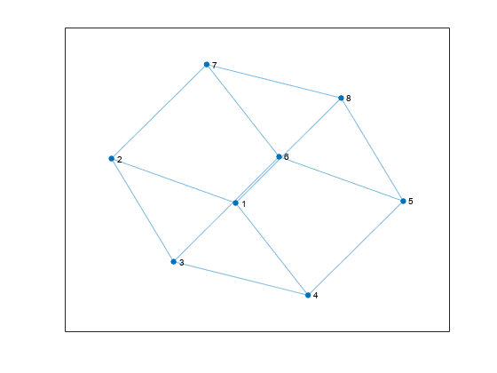
Edge List Graph Construction with Node Names and Edge Weights
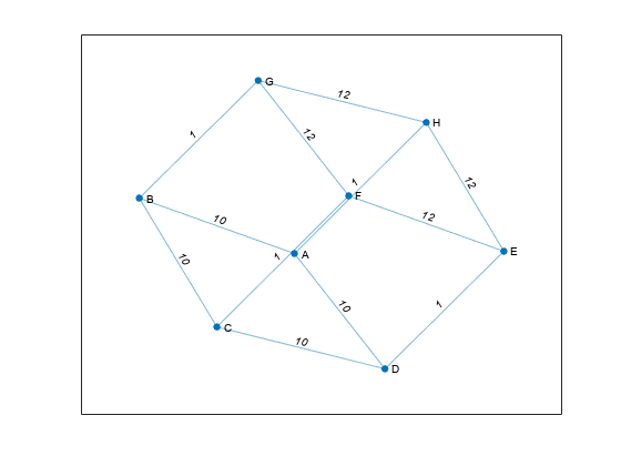
Create and plot a cube graph using a list of the end nodes of each edge. Specify node names and edge weights as separate inputs.
s = [1 1 1 2 2 3 3 4 5 5 6 7]; t = [2 4 8 3 7 4 6 5 6 8 7 8]; weights = [10 10 1 10 1 10 1 1 12 12 12 12]; names = {'A' 'B' 'C' 'D' 'E' 'F' 'G' 'H'}; G = graph(s,t,weights,names)
G = graph with properties:
Edges: [12x2 table]
Nodes: [8x1 table]
plot(G,'EdgeLabel',G.Edges.Weight)
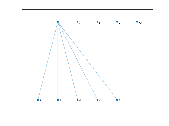
Edge List Construction with Extra Nodes
Create a weighted graph using a list of the end nodes of each edge. Specify that the graph should contain a total of 10 nodes.
s = [1 1 1 1 1]; t = [2 3 4 5 6]; weights = [5 5 5 6 9]; G = graph(s,t,weights,10)
G = graph with properties:
Edges: [5x2 table]
Nodes: [10x0 table]
Plot the graph. The extra nodes are disconnected from the primary connected component.
Add Nodes and Edges to Empty Graph
Create an empty graph object, G.
Add three nodes and three edges to the graph. The corresponding entries in s and t define the end nodes of the graph edges. addedge automatically adds the appropriate nodes to the graph if they are not already present.
s = [1 2 1]; t = [2 3 3]; G = addedge(G,s,t)
G = graph with properties:
Edges: [3x1 table]
Nodes: [3x0 table]
View the edge list. Each row describes an edge in the graph.
ans=3×1 table EndNodes ________
 1    2
 1    3
 2    3
For the best performance, construct graphs all at once using a single call to graph. Adding nodes or edges in a loop can be slow for large graphs.
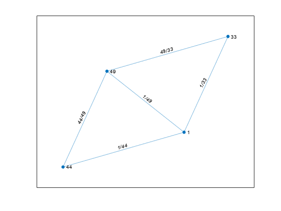
Graph Construction with Tables
Create an edge table that contains the variables EndNodes, Weight, and Code. Then create a node table that contains the variables Name and Country. The variables in each table specify properties of the graph nodes and edges.
s = [1 1 1 2 3]; t = [2 3 4 3 4]; weights = [6 6.5 7 11.5 17]'; code = {'1/44' '1/49' '1/33' '44/49' '49/33'}'; EdgeTable = table([s' t'],weights,code, ... 'VariableNames',{'EndNodes' 'Weight' 'Code'})
EdgeTable=5×3 table
EndNodes Weight Code
________ ______ _________
 1    2         6     {'1/44' }
 1    3       6.5     {'1/49' }
 1    4         7     {'1/33' }
 2    3      11.5     {'44/49'}
 3    4        17     {'49/33'}
names = {'USA' 'GBR' 'DEU' 'FRA'}'; country_code = {'1' '44' '49' '33'}'; NodeTable = table(names,country_code,'VariableNames',{'Name' 'Country'})
NodeTable=4×2 table Name Country _______ _______
{'USA'}    {'1' }
{'GBR'}    {'44'}
{'DEU'}    {'49'}
{'FRA'}    {'33'}
Create a graph using the node and edge tables. Plot the graph using the country codes as node and edge labels.
G = graph(EdgeTable,NodeTable); plot(G,'NodeLabel',G.Nodes.Country,'EdgeLabel',G.Edges.Code)
Extended Capabilities
C/C++ Code Generation
Generate C and C++ code using MATLAB® Coder™.
Usage notes and limitations:
- Node names are not supported. Use node indices instead.
- Sparse inputs are not supported for constructing edge lists.
- Code generation for
graphobjects only supports the following object functions:addedge,addnode,adjacency,conncomp,degree,edgecount,indegree,neighbors,numedges,numnodes,outdegree,outedges,rmnode,rmedge,subgraph. - Saving and loading
graphobjects is not supported. - If a variable-size edge weight is specified during code generation and an empty weight vector is given at runtime, then the
G.Edgestable contains aWeightvariable containing a vector of ones. - You must specify the number and types of the edge and node properties when creating the
graphobjects. You cannot add new variables to the edge and node properties usingaddnodeoraddedge. That is, you cannot add new columns to theG.EdgesandG.Nodestables. - When you construct a
graphobject in MATLAB® and pass it to a MEX function generated using MATLAB Coder™, you cannot add or remove edges or nodes from thegraphobject. - The edge and node properties must be data types that can be stored as variable-size arrays in code generation. For example, the data type cannot be any of these:
- a string array
- a cell array with different sizes on each cell
- a cell array of character vectors converted using
cellstr - a user-defined class
Thread-Based Environment
Run code in the background using MATLAB® backgroundPool or accelerate code with Parallel Computing Toolbox™ ThreadPool.
Version History
Introduced in R2015b
R2019a: Support for categorical node names
Support added for categorical node names as inputs. This enables you to use data that is imported as categorical to create a graph, without the need for data type manipulation.
R2018a: Change in handling of duplicate edges
graph, digraph, andaddedge no longer produce errors when they encounter duplicate edges. Instead, the duplicate edges are added to the graph and the result is a multigraph. The ismultigraph function is useful to detect this situation, andsimplify provides an easy way to remove the extra edges.