subplot - Create axes in tiled positions - MATLAB (original) (raw)

Create axes in tiled positions

Syntax

Description

Note

tiledlayout is recommended oversubplot because it enables you to create layouts with adjustable tile spacing, tiles that reflow according to the size of the figure, and better placed colorbars and legends.

subplot([m](#btw1t4b-1-m),[n](#btw1t4b-1-n),[p](#btw1t4b-1-p)) divides the current figure into an m-by-n grid and creates axes in the position specified by p. MATLAB® numbers subplot positions by row. The first subplot is the first column of the first row, the second subplot is the second column of the first row, and so on. If axes exist in the specified position, then this command makes the axes the current axes.

example

subplot([m](#btw1t4b-1-m),[n](#btw1t4b-1-n),[p](#btw1t4b-1-p),`'replace'`) deletes existing axes in position p and creates new axes.

example

subplot([m](#btw1t4b-1-m),[n](#btw1t4b-1-n),[p](#btw1t4b-1-p),`'align'`) creates new axes so that the plot boxes are aligned. This option is the default behavior.

subplot([m](#btw1t4b-1-m),[n](#btw1t4b-1-n),[p](#btw1t4b-1-p),[ax](#btw1t4b-1-ax)) converts the existing axes, ax, into a subplot in the same figure.

example

subplot(`'Position'`,[pos](#btw1t4b-1-pos)) creates axes in the custom position specified by pos. Use this option to position a subplot that does not align with grid positions. Specify pos as a four-element vector of the form [left bottom width height]. If the new axes overlap existing axes, then the new axes replace the existing axes.

example

subplot(___,[Name,Value](#namevaluepairarguments)) modifies axes properties using one or more name-value pair arguments. Set axes properties after all other input arguments.

[ax](#btw1t4b-1-ax) = subplot(___) creates an Axes object, PolarAxes object, or GeographicAxes object. Use ax to make future modifications to the axes.

example

subplot([ax](#btw1t4b-1-ax)) makes the axes specified by ax the current axes for the parent figure. This option does not make the parent figure the current figure if it is not already the current figure.

example

Examples

collapse all

Upper and Lower Subplots

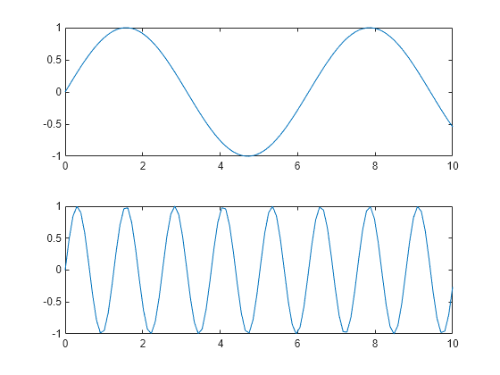
Create a figure with two stacked subplots. Plot a sine wave in each one.

subplot(2,1,1); x = linspace(0,10); y1 = sin(x); plot(x,y1)

subplot(2,1,2); y2 = sin(5*x); plot(x,y2)

Quadrant of Subplots

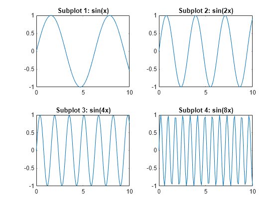
Create a figure divided into four subplots. Plot a sine wave in each one and title each subplot.

subplot(2,2,1) x = linspace(0,10); y1 = sin(x); plot(x,y1) title('Subplot 1: sin(x)')

subplot(2,2,2) y2 = sin(2*x); plot(x,y2) title('Subplot 2: sin(2x)')

subplot(2,2,3) y3 = sin(4*x); plot(x,y3) title('Subplot 3: sin(4x)')

subplot(2,2,4) y4 = sin(8*x); plot(x,y4) title('Subplot 4: sin(8x)')

Subplots with Different Sizes

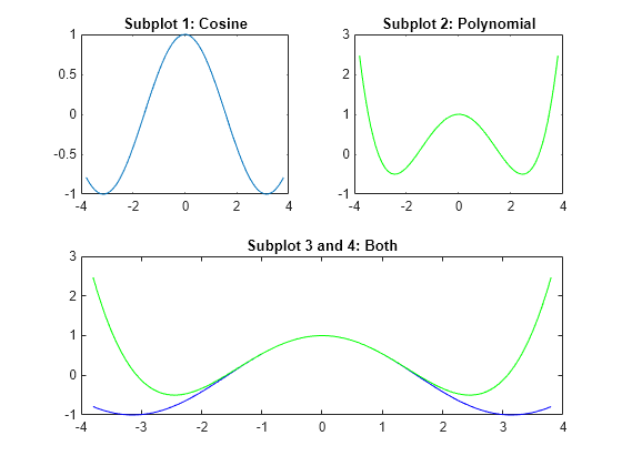
Create a figure containing with three subplots. Create two subplots across the upper half of the figure and a third subplot that spans the lower half of the figure. Add titles to each subplot.

subplot(2,2,1); x = linspace(-3.8,3.8); y_cos = cos(x); plot(x,y_cos); title('Subplot 1: Cosine')

subplot(2,2,2); y_poly = 1 - x.^2./2 + x.^4./24; plot(x,y_poly,'g'); title('Subplot 2: Polynomial')

subplot(2,2,[3,4]); plot(x,y_cos,'b',x,y_poly,'g'); title('Subplot 3 and 4: Both')

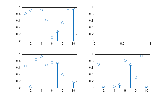
Replace Subplot with Empty Axes

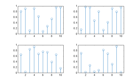
Create a figure with four stem plots of random data. Then replace the second subplot with empty axes.

for k = 1:4 data = rand(1,10); subplot(2,2,k) stem(data) end

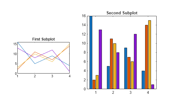
Subplots at Custom Positions

Create a figure with two subplots that are not aligned with grid positions. Specify a custom position for each subplot.

pos1 = [0.1 0.3 0.3 0.3]; subplot('Position',pos1) y = magic(4); plot(y) title('First Subplot')

pos2 = [0.5 0.15 0.4 0.7]; subplot('Position',pos2) bar(y) title('Second Subplot')

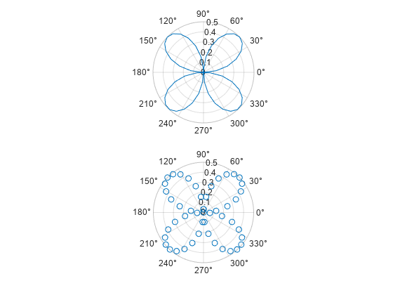
Create Subplots with Polar Axes

Create a figure with two polar axes. Create a polar line chart in the upper subplot and a polar scatter chart in the lower subplot.

figure ax1 = subplot(2,1,1,polaraxes); theta = linspace(0,2*pi,50); rho = sin(theta).*cos(theta); polarplot(ax1,theta,rho)

ax2 = subplot(2,1,2,polaraxes); polarscatter(ax2,theta,rho)

Modify Axes Properties After Creation

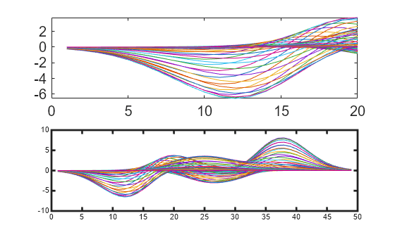
Create a figure with two subplots. Assign the Axes objects to the variables ax1 and ax2. Specify the Axes objects as inputs to the plotting functions to ensure that the functions plot into a specific subplot.

ax1 = subplot(2,1,1); Z = peaks; plot(ax1,Z(1:20,:))

ax2 = subplot(2,1,2);
plot(ax2,Z)

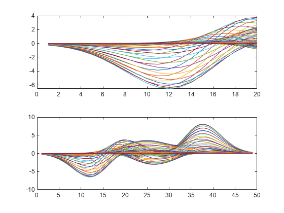
Modify the axes by setting properties of the Axes objects. Change the font size for the upper subplot and the line width for the lower subplot. Some plotting functions set axes properties. Execute plotting functions before specifying axes properties to avoid overriding existing axes property settings. Use dot notation to set properties.

ax1.FontSize = 15; ax2.LineWidth = 2;

Make Subplot the Current Axes

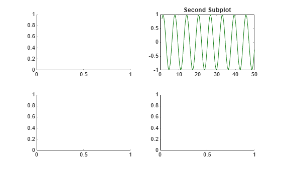
Create a figure with multiple subplots. Store the Axes objects in vector ax. Then make the second subplot the current axes. Create a line chart and change the axis limits for the second subplot. By default, graphics functions target the current axes.

for k = 1:4 ax(k) = subplot(2,2,k); end

subplot(ax(2)) x = linspace(1,50); y = sin(x); plot(x,y,'Color',[0.1, 0.5, 0.1]) title('Second Subplot') axis([0 50 -1 1])

Convert Existing Axes to Subplot

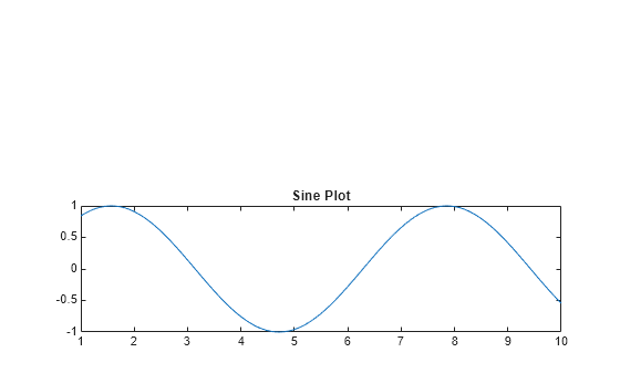
Create a line chart. Then convert the axes so that it is the lower subplot of the figure. The subplot function uses the figure in which the original axes existed.

x = linspace(1,10); y = sin(x); plot(x,y) title('Sine Plot')

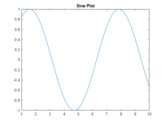
ax = gca; subplot(2,1,2,ax)

Convert Axes in Separate Figures to Subplots

Combine axes that exist in separate figures in a single figure with subplots.

Create two plots in two different figures. Assign the Axes objects to the variables ax1 and ax2. Assign the Legend object to the variablelgd.

figure x = linspace(0,10); y1 = sin(x); plot(x,y1) title('Line Plot 1') ax1 = gca;

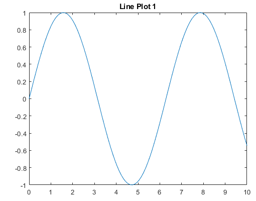
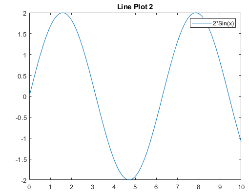
figure y2 = 2sin(x); plot(x,y2) title('Line Plot 2') lgd = legend('2Sin(x)'); ax2 = gca;

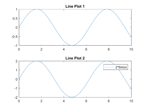
Create copies of the two Axes objects using copyobj. Specify the parents of the copied axes as a new figure. Since legends and colorbars do not get copied with the associated axes, copy the legend with the axes.

fnew = figure; ax1_copy = copyobj(ax1,fnew); subplot(2,1,1,ax1_copy)

copies = copyobj([ax2,lgd],fnew); ax2_copy = copies(1); subplot(2,1,2,ax2_copy)

Input Arguments

collapse all

m — Number of grid rows

1 (default) | positive integer

Number of grid rows, specified as a positive integer.

Data Types: single | double

n — Number of grid columns

1 (default) | positive integer

Number of grid columns, specified as a positive integer.

Data Types: single | double

p — Grid position for new axes

scalar | vector

Grid position for the new axes, specified as a scalar or vector of positive integers.

• If p is a scalar positive integer, then subplot creates a subplot in grid position p.
• If p is a vector of positive integers, then subplot creates a subplot that spans the grid positions listed in p.

Example: subplot(2,3,1) creates a subplot in position 1.

Example: subplot(2,3,[2,5]) creates a subplot spanning positions 2 and 5.

Example: subplot(2,3,[2,6]) creates a subplot spanning positions 2, 3, 5, and 6.

Data Types: single | double

pos — Custom position for new axes

four-element vector

Custom position for the new axes, specified as a four-element vector of the form [left bottom width height].

• The left and bottom elements specify the position of the bottom-left corner of the subplot in relation to the bottom-left corner of the figure.
• The width and height elements specify the subplot dimensions.

Specify values between 0 and 1 that are normalized with respect to the interior of the figure.

Note

When using a script to create subplots, MATLAB does not finalize the Position property value until either a drawnow command is issued or MATLAB returns to await a user command. The Position property value for a subplot is subject to change until the script either refreshes the plot or exits.

Example: subplot('Position',[0.1 0.1 0.45 0.45])

Data Types: single | double

ax — Existing axes to make current or convert to subplot

Axes object | PolarAxes object | GeographicAxes object | graphics object

Existing axes to make current or convert to a subplot, specified as an Axes object, a PolarAxes object, aGeographicAxes object, or a graphics object with an PositionConstraint property, such as aHeatmapChart object.

To create empty polar or geographic axes in a subplot position, specify ax as the polaraxes or geoaxes function. For example,subplot(2,1,2,polaraxes).

Name-Value Arguments

Specify optional pairs of arguments asName1=Value1,...,NameN=ValueN, where Name is the argument name and Value is the corresponding value. Name-value arguments must appear after other arguments, but the order of the pairs does not matter.

Before R2021a, use commas to separate each name and value, and enclose Name in quotes.

Example: subplot(m,n,p,'XGrid','on')

Some plotting functions override property settings. Consider setting axes properties after plotting. The properties you can set depend on the type of axes:

• For Cartesian axes, see Axes Properties.
• For polar axes, see PolarAxes Properties.
• For geographic axes, see GeographicAxes Properties.

Tips

• To clear the contents of the figure, use clf. For example, you might clear the existing subplot layout from the figure before creating a new subplot layout.
• To overlay axes, use the axes command instead. The subplot function deletes existing axes that overlap new axes. For example, subplot('Position',[.35 .35 .3 .3]) deletes any underlying axes, but axes('Position',[.35 .35 .3 .3]) positions new axes in the middle of the figure without deleting underlying axes.
• subplot(111) is an exception and not identical in behavior to subplot(1,1,1). For reasons of backwards compatibility, subplot(111) is a special case of subplot that does not immediately create axes, but sets up the figure so that the next graphics command executes clf reset. The next graphics command deletes all the figure children and creates new axes in the default position. subplot(111) does not return an Axes object and an error occurs if code specifies a return argument.

Alternative Functionality

Use the tiledlayout and nexttile functions to create a configurable tiling of plots. The configuration options include:

• Control over the spacing between the plots and around the edges of the layout
• An option for a shared title at the top of the layout
• Options for shared _x_- and _y_-axis labels
• An option to control whether the tiling has a fixed size or variable size that can reflow

For more information, see Combine Multiple Plots.

Version History

Introduced before R2006a