Data Analysis with Python (original) (raw)

Last Updated : 18 Apr, 2026

Data Analysis involves collecting, transforming and organizing data to generate insights, support decision making and solve business problems.

• Helps in making informed, data driven decisions
• Identifies patterns and trends for better predictions
• Supports solving real world business problems
• Converts raw data into meaningful insights

Analyzing Numerical Data with NumPy

NumPy is a Python library used for fast and efficient numerical computations. It provides multidimensional arrays and built in functions that simplify data analysis, mathematical operations and large scale data processing.

Arrays in NumPy

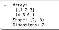
NumPy arrays store elements of the same data type and support multiple dimensions. The number of dimensions is called rank and the size of each dimension is called shape.

Python `

import numpy as np

arr = np.array([[1, 2, 3], [4, 5, 6]]) print("Array:\n", arr) print("Shape:", arr.shape) print("Dimensions:", arr.ndim)

`

**Output:

Output

Creating NumPy Arrays

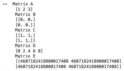
Arrays can be created using lists, tuples or built in functions like zeros, ones, arange and empty.

Python `

a = np.array([1, 2, 3]) b = np.zeros((2, 2)) c = np.ones((2, 2)) d = np.arange(0, 10, 2) e = np.empty((2, 2), dtype=int)

print("Matrix A \n", a, "\n Matrix B \n", b, "\n Matrix C \n", c, "\n Matrix D \n", d, "\n Matrix E \n", e)

`

**Output:

Output

Operations on Numpy Arrays

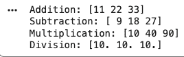
NumPy allows efficient element wise operations on arrays, making numerical computations faster and more optimized compared to traditional Python methods.

• **Addition: Adds corresponding elements of two arrays
• **Subtraction: Subtracts elements of one array from another
• **Multiplication: Performs element wise multiplication
• **Division: Divides elements of one array by another Python `

import numpy as np

a = np.array([10, 20, 30]) b = np.array([1, 2, 3])

print("Addition:", a + b) print("Subtraction:", a - b) print("Multiplication:", a * b) print("Division:", a / b)

`

**Output:

Arithmetic Operations on Arrays

NumPy Array Indexing

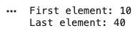
Indexing is used to access individual elements in an array using their position. It works similarly to Python lists but is more useful for multi dimensional data.

Python `

arr = np.array([10, 20, 30, 40])

print("First element:", arr[0]) print("Last element:", arr[-1])

`

**Output:

Array Indexing

NumPy Array Slicing

Slicing allows accessing a range of elements from an array. It is useful for working with subsets of data.

Python `

arr = np.array([10, 20, 30, 40, 50])

print("Slice (1 to 3):", arr[1:4]) print("First three elements:", arr[:3])

`

**Output:

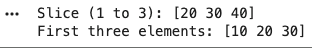
Output

NumPy Array Broadcasting

Broadcasting allows operations between arrays of different shapes without explicitly resizing them, improving efficiency and reducing code complexity.

Python `

arr = np.array([1, 2, 3])

print("Add scalar:", arr + 5)

b = np.array([[1], [2], [3]]) c = np.array([10, 20, 30])

print("Broadcasting result:\n", b + c)

`

**Output:

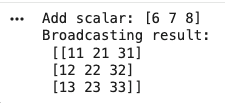
Broadcasting

Analyzing Data Using Pandas

Pandas is a Python library used for handling structured (relational or labeled) data. Built on top of NumPy, it provides flexible data structures and tools for data manipulation, analysis and time series operations.

• Used for working with structured and tabular data
• Built on top of NumPy for high performance
• Supports data cleaning, transformation and analysis

Series in Pandas

A Series is a one dimensional labeled array capable of holding any data type (integers, strings, floats, etc.). Each element has an associated index.

• Represents a single column of data
• Supports indexing and labeling
• Can store different data types Python `

import pandas as pd

data = [10, 20, 30, 40] series = pd.Series(data)

print(series) print("First element:", series[0])

`

**Output:

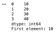
Series

**DataFrame in Pandas

A DataFrame is a two dimensional labeled data structure with rows and columns, similar to a table or spreadsheet.

• Represents tabular data (rows and columns)
• Each column can have a different data type
• Most commonly used Pandas structure Python `

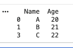
import pandas as pd

data = { "Name": ["A", "B", "C"], "Age": [20, 21, 22] }

df = pd.DataFrame(data)

print(df) print("Column Access:\n", df["Name"])

`

**Output:

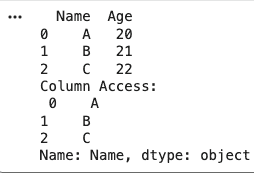
DataFrame

Pandas CRUD Operations

Pandas allows easy Create, Read, Update and Delete operations on data stored in CSV files, making it practical for real-world datasets. It is known as CRUD Oprations.

• **Create: Create and save a DataFrame as a CSV file
• **Read: Load data from a CSV file
• **Update: Modify values or add new columns
• **Delete: Remove rows or columns Python `

import pandas as pd

data = {"Name": ["A", "B", "C"], "Age": [20, 21, 22]} df = pd.DataFrame(data) df.to_csv("data.csv", index=False)

df = pd.read_csv("data.csv") print("Read:\n", df)

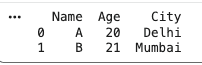
df["Age"] = df["Age"] + 1 df["City"] = ["Delhi", "Mumbai", "Pune"] print("\nUpdate:\n", df)

df = df.drop("City", axis=1)
df = df.drop(0, axis=0)
print("\nDelete:\n", df)

`

**Output:

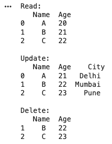
CRUD Operations on a Dataset

Exploratory Data Analysis (EDA)

1. Data Inspection

Pandas provides quick methods to understand the structure, summary and content of a dataset. These functions help in exploring data before analysis.

• **info(): Displays dataset structure, column names, data types and non null values
• **describe()****:** Shows statistical summary like mean, min, max and standard deviation
• **value_counts(): Counts frequency of unique values in a column
• **head(): Displays first few rows of the dataset
• **tail():Displays last few rows of the dataset Python `

import pandas as pd

data = { "Name": ["A", "B", "C", "A", "B"], "Age": [20, 21, 22, 20, 21] } df = pd.DataFrame(data)

print("Info:") print(df.info())

print("\nDescribe:\n", df.describe())

print("\nValue Counts:\n", df["Name"].value_counts())

print("\nHead:\n", df.head())

print("\nTail:\n", df.tail())

`

**Output:

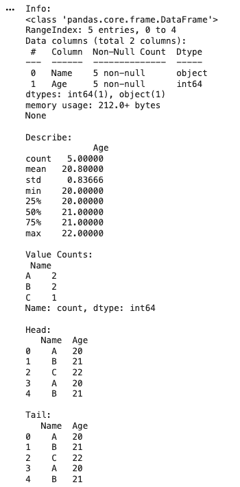
Output

2. Data Manipulation in Pandas

Pandas provides multiple operations to efficiently select, organize and transform data for analysis.

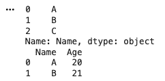
**Indexing and Selection

Indexing and Selection are used to access specific rows, columns or subsets of data.

Python `

import pandas as pd

df = pd.DataFrame({ "Name": ["A", "B", "C"], "Age": [20, 21, 22] })

print(df["Name"])
print(df.iloc[0:2])

`

**Output:

Output

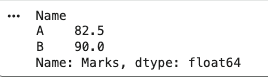
**Grouping and Aggregation

Grouping and Aggregation Groups data based on a column and applies aggregate functions like mean, sum, etc.

Python `

import pandas as pd

df = pd.DataFrame({ "Name": ["A", "B", "A"], "Marks": [80, 90, 85] })

print(df.groupby("Name")["Marks"].mean())

`

**Output:

Output

**Merging and Joining

Merging and Joining combines multiple DataFrames based on common columns.

Python `

import pandas as pd

df1 = pd.DataFrame({"Name": ["A", "B"], "Age": [20, 21]}) df2 = pd.DataFrame({"Name": ["A", "B"], "City": ["Delhi", "Mumbai"]})

print(pd.merge(df1, df2, on="Name"))

`

**Output:

Output

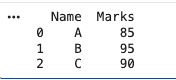
**Sort

Sorts data based on column values.

Python `

import pandas as pd

df = pd.DataFrame({ "Name": ["A", "B", "C"], "Marks": [85, 95, 90] })

print(df.sort_values(by="Marks", ascending=False))

`

**Output:

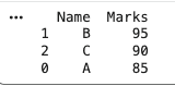
Output

**Filter

Filter selects data based on conditions.

Python `

import pandas as pd

df = pd.DataFrame({ "Name": ["A", "B", "C"], "Marks": [85, 95, 90] })

print(df[df["Marks"] > 88])

`

**Output:

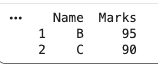
Output

**set_index

Sets a column as the index of the DataFrame.

Python `

import pandas as pd

df = pd.DataFrame({ "Name": ["A", "B", "C"], "Marks": [85, 95, 90] })

print(df.set_index("Name"))

`

**Output:

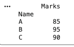
Output

**reset_index

Resets the index back to default numeric indexing.

Python `

import pandas as pd

df = pd.DataFrame({ "Name": ["A", "B", "C"], "Marks": [85, 95, 90] }).set_index("Name")

print(df.reset_index())

`

**Output:

Output

3. Working With Missing Data

Working with missing data is a key step in EDA to ensure data quality and accurate analysis. It involves identifying missing values and applying appropriate techniques to handle them without affecting results.

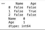
**Checking Missing Data

Used to detect null values present in the dataset.

Python `

import pandas as pd

df = pd.DataFrame({ "Name": ["A", "B", "C"], "Age": [20, None, 22] })

print(df.isnull())
print(df.isnull().sum())

`

**Output:

Output

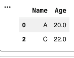
**Dropping Missing Values

There are different methods to handle missing data based on requirements, here we just drop the missing values.

Python `

import pandas as pd

df = pd.DataFrame({ "Name": ["A", "B", "C"], "Age": [20, None, 22] })

print(df.dropna())

df["Age"].fillna(df["Age"].mean(), inplace=True) print(df)

`

**Output:

Output

4. Checking and Handling Duplicate Values

Duplicate values can lead to incorrect analysis and biased results. Identifying and removing duplicates is an important step in data cleaning during EDA.

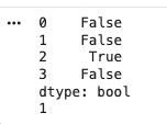
**Checking Duplicate Values

Used to detect duplicate rows in the dataset.

Python `

import pandas as pd

df = pd.DataFrame({ "Name": ["A", "B", "A", "C"], "Age": [20, 21, 20, 22] })

print(df.duplicated())
print(df.duplicated().sum())

`

**Output:

Output

**Handling Duplicate Values

Remove duplicate rows to clean the dataset.

Python `

import pandas as pd

df = pd.DataFrame({ "Name": ["A", "B", "A", "C"], "Age": [20, 21, 20, 22] })

df_clean = df.drop_duplicates() print(df_clean)

`

**Output:

Output

5. Outlier Detection and Handling

Outliers are extreme values that differ significantly from other data points. Detecting and handling them is important to improve data quality and model performance during EDA.

**IQR (Interquartile Range) Method

Outliers are values below Q1 - 1.5 IQR or above Q3 + 1.5 IQR.

Python `

import pandas as pd

df = pd.DataFrame({ "Values": [10, 12, 14, 15, 100] })

Q1 = df["Values"].quantile(0.25) Q3 = df["Values"].quantile(0.75) IQR = Q3 - Q1

outliers = df[(df["Values"] < Q1 - 1.5IQR) | (df["Values"] > Q3 + 1.5IQR)] print("Outliers:\n", outliers)

`

**Output:

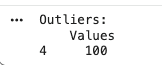
Output

**Z-Score Method

Outliers are values with Z-score greater than 3 or less than -3.

Python `

import pandas as pd import numpy as np

df = pd.DataFrame({ "Values": [10, 12, 14, 15, 100] })

mean = np.mean(df["Values"]) std = np.std(df["Values"])

df["Z_score"] = (df["Values"] - mean) / std outliers = df[df["Z_score"].abs() > 3]

print("Outliers:\n", outliers)

`

**Output:

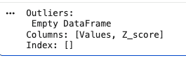
No outliers in the dataset

**Handling Outliers

Outliers can be handled by removing or capping depending on the use case.

Python `

import pandas as pd

df = pd.DataFrame({ "Values": [10, 12, 14, 15, 100] })

Q1 = df["Values"].quantile(0.25) Q3 = df["Values"].quantile(0.75) IQR = Q3 - Q1

df_clean = df[(df["Values"] >= Q1 - 1.5IQR) & (df["Values"] <= Q3 + 1.5IQR)] print("After Removing Outliers:\n", df_clean)

`

**Output:

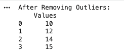
Output

6. Data Visualization Using Matplotlib

Matplotlib is a widely used Python library for creating visualizations and graphs. It helps in understanding patterns, trends, and relationships in data through visual representation during EDA.

• Used to create plots like line charts, bar graphs, histograms and scatter plots
• Helps in identifying trends, distributions and outliers
• Works well with NumPy and Pandas data

**Pyplot

Pyplot is a Matplotlib module that provides a simple interface to create and customize plots. It helps in generating figures, adding labels, and displaying visualizations.

Python `

import matplotlib.pyplot as plt

plt.plot([1, 2, 3, 4], [1, 4, 9, 16]) plt.axis([0, 6, 0, 20]) plt.show()

`

**Output:

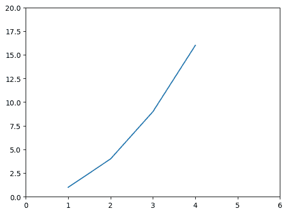
Output

**Bar chart

A bar chart is used to compare values across different categories using rectangular bars. The height or length of each bar represents the value of that category.

• Used for comparing discrete categories
• Can be plotted vertically or horizontally
• Created using bar() method Python `

import matplotlib.pyplot as plt from sklearn.datasets import load_iris import pandas as pd

iris = load_iris() df = pd.DataFrame(iris.data, columns=iris.feature_names) df["target"] = iris.target

counts = df["target"].value_counts()

plt.bar(counts.index, counts.values) plt.title("Bar Chart (Iris Dataset)") plt.xlabel("Class") plt.ylabel("Count") plt.show()

`

**Output:

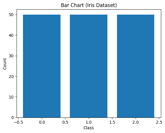
Bar chart

**Histograms

A histogram is used to show the distribution of data by grouping values into bins (ranges). The X-axis represents the bins, and the Y-axis shows the frequency of values in each bin.

• Used to understand data distribution
• Groups data into non-overlapping intervals (bins)
• Created using hist() method Python `

import matplotlib.pyplot as plt from sklearn.datasets import load_iris import pandas as pd

iris = load_iris() df = pd.DataFrame(iris.data, columns=iris.feature_names)

plt.hist(df["sepal length (cm)"], bins=10) plt.title("Histogram (Iris Dataset)") plt.xlabel("Sepal Length") plt.ylabel("Frequency") plt.show()

`

**Output:

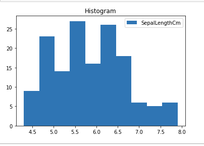
Histplot using matplotlib library

**Scatter Plot

Scatter plots are used to observe relationship between variables and uses dots to represent the relationship between them. The scatter() method in the matplotlib library is used to draw a scatter plot.

Python `

import matplotlib.pyplot as plt from sklearn.datasets import load_iris import pandas as pd

iris = load_iris() df = pd.DataFrame(iris.data, columns=iris.feature_names) df["species"] = iris.target

plt.scatter(df["sepal length (cm)"], df["sepal width (cm)"])

plt.title("Scatter Plot (Iris Dataset)") plt.xlabel("Sepal Length") plt.ylabel("Sepal Width")

plt.show()

`

**Output:

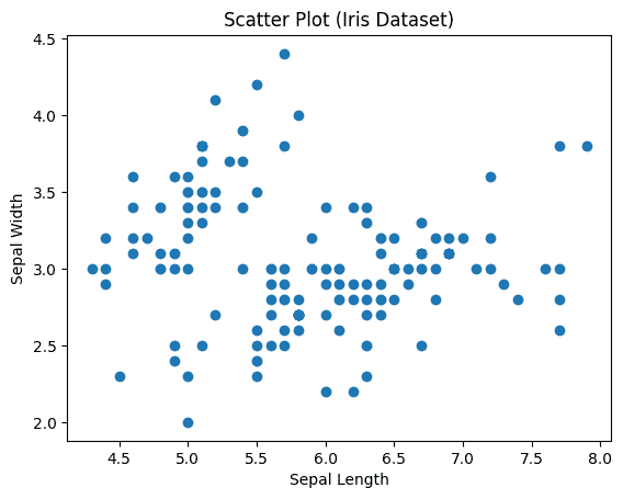
Scatter plot using matplotlib library

**Box Plot

A boxplot (box-and-whisker plot) is used to visualize data distribution and identify outliers using quartiles.The minimum is shown at the far left of the chart, at the end of the left ‘whisker’

• First quartile, Q1, is the far left of the box (left whisker)
• The median is shown as a line in the center of the box
• Third quartile, Q3, shown at the far right of the box (right whisker)
• The maximum is at the far right of the box Python `

import matplotlib.pyplot as plt from sklearn.datasets import load_iris import pandas as pd

iris = load_iris() df = pd.DataFrame(iris.data, columns=iris.feature_names)

plt.boxplot(df["sepal width (cm)"], labels=["Sepal Width"])

plt.title("Box Plot (Iris Dataset)") plt.ylabel("Value")

plt.show()

`

**Output:

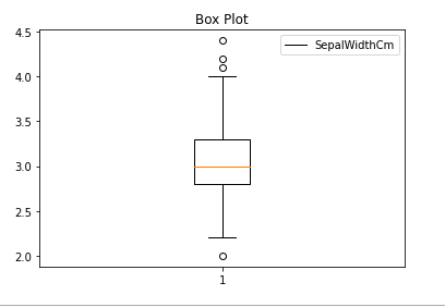
Boxplot using matplotlib library

**Correlation Heatmaps

A correlation heatmap is a visual tool that shows relationships between variables using colors. It is based on a correlation matrix, where each cell represents how strongly two variables are related.

• Uses colors to represent correlation values (-1 to +1)
• Helps identify patterns, relationships, and dependencies
• Created using corr() to compute correlation matrix
• Color intensity shows strength of relationship
• Works only with numerical data Python `

import matplotlib.pyplot as plt from sklearn.datasets import load_iris import pandas as pd

iris = load_iris() df = pd.DataFrame(iris.data, columns=iris.feature_names)

corr = df.corr()

plt.imshow(corr, cmap='autumn', interpolation='nearest')

plt.title("Correlation Heatmap") plt.colorbar()
plt.xticks(range(len(corr.columns)), corr.columns, rotation=45) plt.yticks(range(len(corr.columns)), corr.columns)

plt.show()

`

**Output:

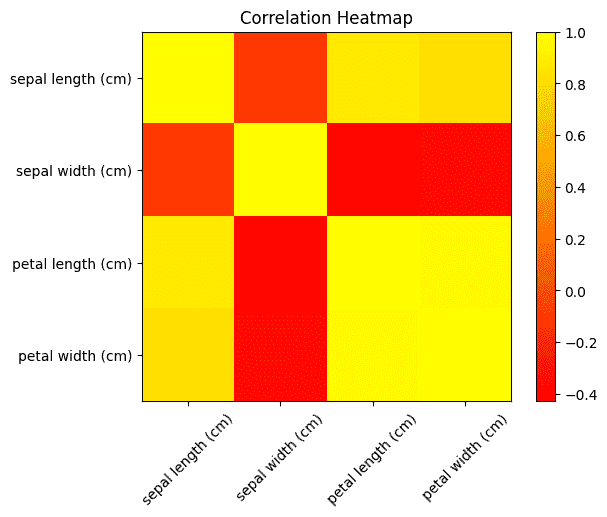
Correlation Heatmap

7. Data Visualization using Seaborn

Seaborn is a high level visualization library built on Matplotlib that provides more attractive and informative statistical plots.

• Better styling and built in themes
• Simplifies complex visualizations
• Works directly with Pandas DataFrames

**Scatter Plot

Python `

import seaborn as sns import matplotlib.pyplot as plt from sklearn.datasets import load_iris import pandas as pd

iris = load_iris() df = pd.DataFrame(iris.data, columns=iris.feature_names) df["species"] = iris.target

sns.scatterplot(x="sepal length (cm)", y="sepal width (cm)", hue="species", data=df)

plt.title("Seaborn Scatter Plot") plt.show()

`

**Output:

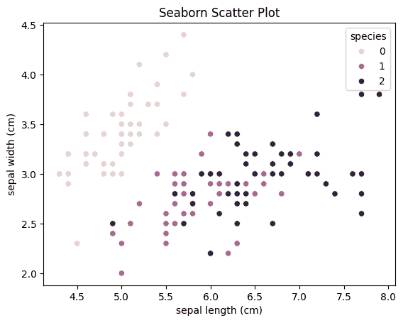
Seaborn Scatter plot